HOUSING PRICE PREDICTION

notebook by Rayen Feng Project start: July 9, 2022 Project end: June 6, 2023

There was a really long break in between this :)

This notebook intends to be for more or less my self learning. Therefore, I will mostly explain the concepts to myself throughout this notebook.

The problem and goal

The goal of this project is to use machine learning techniques to predict the housing prices of a given house. We’re given a set of training data as well as testing data to accomplish this task.

The outline

Here are the steps that this analysis will take.

Understand the data - this step will focus on looking at the varibles in the dataset and draft out some initial thoughts on what variables correlate to sale price. This will involve looking at each varibale and filtering out the useful ones from the one with little relevance.
Data Cleaning - once all the variables are skimmed through, some data cleaning will be done. This includes dealing with missing values, duplicate numbers, and outliers in any way.
Buidlding models - once the data is clean, we can start building some models. Each one of these steps will most likely be refined as work is done, but this is the overall approach for it. We will use the training models to develop a model and use the test dataset to test it.

To answer the first question:

what variables are in relationship with saleprice?

import pandas as pd
import matplotlib.pyplot as plt
import seaborn as sns
import numpy as np
from scipy.stats import norm
from sklearn.preprocessing import StandardScaler
from scipy import stats
import warnings
warnings.filterwarnings('ignore')
%matplotlib inline
sns.set_style("whitegrid")

# import data
df_train = pd.read_csv('../input/house-prices-advanced-regression-techniques/train.csv')
df_test = pd.read_csv('../input/house-prices-advanced-regression-techniques/test.csv')
df_sample = pd.read_csv('../input/house-prices-advanced-regression-techniques/sample_submission.csv')

print(df_train.columns)
df_train.head()

Index(['Id', 'MSSubClass', 'MSZoning', 'LotFrontage', 'LotArea', 'Street',
       'Alley', 'LotShape', 'LandContour', 'Utilities', 'LotConfig',
       'LandSlope', 'Neighborhood', 'Condition1', 'Condition2', 'BldgType',
       'HouseStyle', 'OverallQual', 'OverallCond', 'YearBuilt', 'YearRemodAdd',
       'RoofStyle', 'RoofMatl', 'Exterior1st', 'Exterior2nd', 'MasVnrType',
       'MasVnrArea', 'ExterQual', 'ExterCond', 'Foundation', 'BsmtQual',
       'BsmtCond', 'BsmtExposure', 'BsmtFinType1', 'BsmtFinSF1',
       'BsmtFinType2', 'BsmtFinSF2', 'BsmtUnfSF', 'TotalBsmtSF', 'Heating',
       'HeatingQC', 'CentralAir', 'Electrical', '1stFlrSF', '2ndFlrSF',
       'LowQualFinSF', 'GrLivArea', 'BsmtFullBath', 'BsmtHalfBath', 'FullBath',
       'HalfBath', 'BedroomAbvGr', 'KitchenAbvGr', 'KitchenQual',
       'TotRmsAbvGrd', 'Functional', 'Fireplaces', 'FireplaceQu', 'GarageType',
       'GarageYrBlt', 'GarageFinish', 'GarageCars', 'GarageArea', 'GarageQual',
       'GarageCond', 'PavedDrive', 'WoodDeckSF', 'OpenPorchSF',
       'EnclosedPorch', '3SsnPorch', 'ScreenPorch', 'PoolArea', 'PoolQC',
       'Fence', 'MiscFeature', 'MiscVal', 'MoSold', 'YrSold', 'SaleType',
       'SaleCondition', 'SalePrice'],
      dtype='object')

	Id	MSSubClass	MSZoning	LotFrontage	LotArea	Street	Alley	LotShape	LandContour	Utilities	...	PoolQC	Fence	MiscFeature	MoSold	YrSold	SaleType	SaleCondition	SalePrice
0	1	60	RL	65.0	8450	Pave	NaN	Reg	Lvl	AllPub	...	NaN	NaN	NaN	2	2008	WD	Normal	208500
1	2	20	RL	80.0	9600	Pave	NaN	Reg	Lvl	AllPub	...	NaN	NaN	NaN	5	2007	WD	Normal	181500
2	3	60	RL	68.0	11250	Pave	NaN	IR1	Lvl	AllPub	...	NaN	NaN	NaN	9	2008	WD	Normal	223500
3	4	70	RL	60.0	9550	Pave	NaN	IR1	Lvl	AllPub	...	NaN	NaN	NaN	2	2006	WD	Abnorml	140000
4	5	60	RL	84.0	14260	Pave	NaN	IR1	Lvl	AllPub	...	NaN	NaN	NaN	12	2008	WD	Normal	250000

5 rows × 81 columns

A quick dive into types of data and how to represent it

OK, we see that the overall condition scatter plot doesn’t really tell us anything, or rather, it’s really hard to tell what is being said in this graph. To better visualize this, we first need to understand some different types of data and the best way to represent each type. You can refer to the image below as a reference as I go over these concepts.

There are two overall types of data. Qualitative and Quantitative.

Quantitative - types of data that can be measured with numbers
Qualitative - also known as categorical data, measures the qualitity of things, and cannot be measured with numbers

Okay, but what about the oveall condition? by definition, this is a type of qaltiative data because it describes the quality of the house, but it’s also on a scale of 1 to 10, what does this mean? does it make this quantitative?

In this case, the qualitative/categorical data can be represented into two sub-categories. The first of which is Nominal data, and the other is ordinal data. A good way to remember the difference is that ordinal data has natural order, where nominal does not. In this case, the overal condition of the house is ordinal data, the qualitiy of the house can be ranked in terms of 1 to 10. Something like the lot shape would be nominal data, it can be categorized into regualar, iregular 1 or irregular 2, but doesn’t have any order to it.

Quantitative continuous vs discrete

This one’s easier to understand, discrete data just means that it’s a whole number, or no numbers inbetween. For example, number of cars would be discreete as you can’t have 1.24 cars, and lot size would be continuous because you can have a 120 sqft, 121 sqft or a 120.546 sqft area.

If you’d like you can read more here

# extracting numerical data columns
quan_cols = list(df_train.describe().columns)
qual_cols= [x for x in list(df_train.columns) if x not in quan_cols]

print("\n ------ Quantatative data ---------\n")
print(quan_cols)
print("\n ------ Qualatative data ---------\n")
print(qual_cols)


# explore quant data, find most relavant
# explore qual data find most relavant 
# numerize qual data 
# split again into train test, then plug into ML and then pray 
# use anime list as reference 
# cross validate it 
# check results with test data 

 ------ Quantatative data ---------

['Id', 'MSSubClass', 'LotFrontage', 'LotArea', 'OverallQual', 'OverallCond', 'YearBuilt', 'YearRemodAdd', 'MasVnrArea', 'BsmtFinSF1', 'BsmtFinSF2', 'BsmtUnfSF', 'TotalBsmtSF', '1stFlrSF', '2ndFlrSF', 'LowQualFinSF', 'GrLivArea', 'BsmtFullBath', 'BsmtHalfBath', 'FullBath', 'HalfBath', 'BedroomAbvGr', 'KitchenAbvGr', 'TotRmsAbvGrd', 'Fireplaces', 'GarageYrBlt', 'GarageCars', 'GarageArea', 'WoodDeckSF', 'OpenPorchSF', 'EnclosedPorch', '3SsnPorch', 'ScreenPorch', 'PoolArea', 'MiscVal', 'MoSold', 'YrSold', 'SalePrice']

 ------ Qualatative data ---------

['MSZoning', 'Street', 'Alley', 'LotShape', 'LandContour', 'Utilities', 'LotConfig', 'LandSlope', 'Neighborhood', 'Condition1', 'Condition2', 'BldgType', 'HouseStyle', 'RoofStyle', 'RoofMatl', 'Exterior1st', 'Exterior2nd', 'MasVnrType', 'ExterQual', 'ExterCond', 'Foundation', 'BsmtQual', 'BsmtCond', 'BsmtExposure', 'BsmtFinType1', 'BsmtFinType2', 'Heating', 'HeatingQC', 'CentralAir', 'Electrical', 'KitchenQual', 'Functional', 'FireplaceQu', 'GarageType', 'GarageFinish', 'GarageQual', 'GarageCond', 'PavedDrive', 'PoolQC', 'Fence', 'MiscFeature', 'SaleType', 'SaleCondition']

Exploring Quantataive Data

The Quantatative data will be explored first. First, variables expected to have an impact will be plotted first. Then a heatmap using pearson and spearman correlation will be plotted to determine which variables have the highest correlation with the sale price. First, taking a look at the properties of sales_price

display(df_train.describe().transpose())

	count	mean	std	min	25%	50%	75%	max
Id	1460.0	730.500000	421.610009	1.0	365.75	730.5	1095.25	1460.0
MSSubClass	1460.0	56.897260	42.300571	20.0	20.00	50.0	70.00	190.0
LotFrontage	1201.0	70.049958	24.284752	21.0	59.00	69.0	80.00	313.0
LotArea	1460.0	10516.828082	9981.264932	1300.0	7553.50	9478.5	11601.50	215245.0
OverallQual	1460.0	6.099315	1.382997	1.0	5.00	6.0	7.00	10.0
OverallCond	1460.0	5.575342	1.112799	1.0	5.00	5.0	6.00	9.0
YearBuilt	1460.0	1971.267808	30.202904	1872.0	1954.00	1973.0	2000.00	2010.0
YearRemodAdd	1460.0	1984.865753	20.645407	1950.0	1967.00	1994.0	2004.00	2010.0
MasVnrArea	1452.0	103.685262	181.066207	0.0	0.00	0.0	166.00	1600.0
BsmtFinSF1	1460.0	443.639726	456.098091	0.0	0.00	383.5	712.25	5644.0
BsmtFinSF2	1460.0	46.549315	161.319273	0.0	0.00	0.0	0.00	1474.0
BsmtUnfSF	1460.0	567.240411	441.866955	0.0	223.00	477.5	808.00	2336.0
TotalBsmtSF	1460.0	1057.429452	438.705324	0.0	795.75	991.5	1298.25	6110.0
1stFlrSF	1460.0	1162.626712	386.587738	334.0	882.00	1087.0	1391.25	4692.0
2ndFlrSF	1460.0	346.992466	436.528436	0.0	0.00	0.0	728.00	2065.0
LowQualFinSF	1460.0	5.844521	48.623081	0.0	0.00	0.0	0.00	572.0
GrLivArea	1460.0	1515.463699	525.480383	334.0	1129.50	1464.0	1776.75	5642.0
BsmtFullBath	1460.0	0.425342	0.518911	0.0	0.00	0.0	1.00	3.0
BsmtHalfBath	1460.0	0.057534	0.238753	0.0	0.00	0.0	0.00	2.0
FullBath	1460.0	1.565068	0.550916	0.0	1.00	2.0	2.00	3.0
HalfBath	1460.0	0.382877	0.502885	0.0	0.00	0.0	1.00	2.0
BedroomAbvGr	1460.0	2.866438	0.815778	0.0	2.00	3.0	3.00	8.0
KitchenAbvGr	1460.0	1.046575	0.220338	0.0	1.00	1.0	1.00	3.0
TotRmsAbvGrd	1460.0	6.517808	1.625393	2.0	5.00	6.0	7.00	14.0
Fireplaces	1460.0	0.613014	0.644666	0.0	0.00	1.0	1.00	3.0
GarageYrBlt	1379.0	1978.506164	24.689725	1900.0	1961.00	1980.0	2002.00	2010.0
GarageCars	1460.0	1.767123	0.747315	0.0	1.00	2.0	2.00	4.0
GarageArea	1460.0	472.980137	213.804841	0.0	334.50	480.0	576.00	1418.0
WoodDeckSF	1460.0	94.244521	125.338794	0.0	0.00	0.0	168.00	857.0
OpenPorchSF	1460.0	46.660274	66.256028	0.0	0.00	25.0	68.00	547.0
EnclosedPorch	1460.0	21.954110	61.119149	0.0	0.00	0.0	0.00	552.0
3SsnPorch	1460.0	3.409589	29.317331	0.0	0.00	0.0	0.00	508.0
ScreenPorch	1460.0	15.060959	55.757415	0.0	0.00	0.0	0.00	480.0
PoolArea	1460.0	2.758904	40.177307	0.0	0.00	0.0	0.00	738.0
MiscVal	1460.0	43.489041	496.123024	0.0	0.00	0.0	0.00	15500.0
MoSold	1460.0	6.321918	2.703626	1.0	5.00	6.0	8.00	12.0
YrSold	1460.0	2007.815753	1.328095	2006.0	2007.00	2008.0	2009.00	2010.0
SalePrice	1460.0	180921.195890	79442.502883	34900.0	129975.00	163000.0	214000.00	755000.0

About Pearson Correlation

looking at the list of all the variables, we can go through them one by one and see which ones might have a chance of influencing the price of the house, and add those to the list of varibables, however, that’s more work than I would like to do. I want to take a detailed look of the data after I do a quick sweep through.

A better method instead of looking at each individual variable is to have python look at it for us instead. The question is how do we do this? well, there’s a good function that does it for me. it’s the ‘.corr’ function, which probably stands for correlation. The documentenation uses a pairwise correlation of columns, but what does this mean?

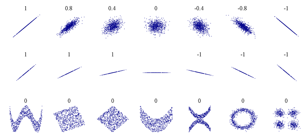
In summary, pairwise correlation uses Pearson’s correlation coefficient (r), which basically is a number from -1 to 1 which shows how direct the relationship is between two variables. A sample scale would be:

weak 0 < r < 0.3
moderate 0.3 < r < 0.6
strong 0.7 < r < 1.0

Of course a strong negative relationship is denoted from 0 to -1. In our case, for example, a coefficent of 0.95 for floor area to sales price could indicate a good correlation between the two variables, and would be something to include in the model.

If you want further reading, you can check out this article from towardsdatascience which covers how you can use seaborn to visualize this

The image below helped the understanding of this concept better. However, something to be weary of is not to confuse this with slope

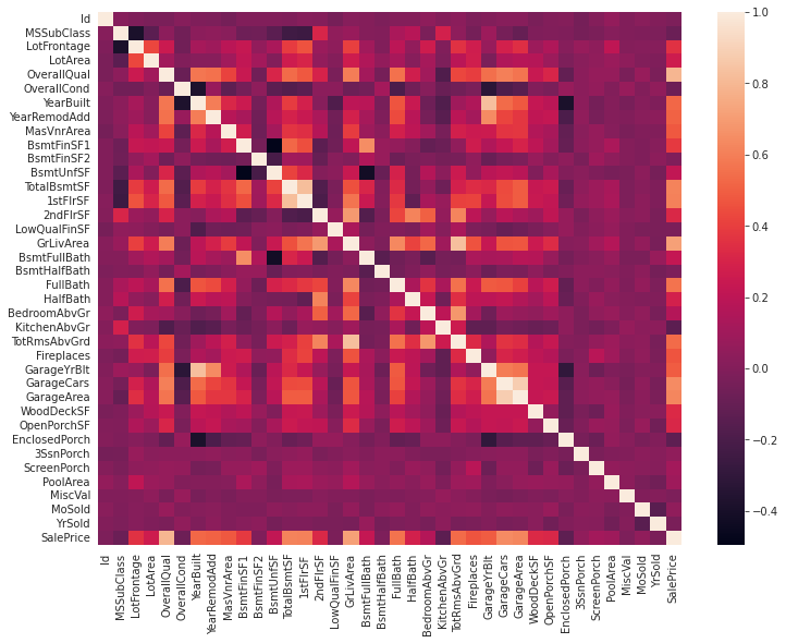
methods = 'pearson'

houses_corrmat = df_train.corr(method= methods)
plt.subplots(figsize=(12, 9))
sns.heatmap(houses_corrmat)

<AxesSubplot:>

png

# extract the column names of the variables with the highest correlation with sale price 
k = 10 
cols_top_ten = houses_corrmat.nlargest(k,'SalePrice')['SalePrice'].index
corrmat_p_top_10 = df_train[cols_top_ten].corr()
corrmat_p_top_10

	SalePrice	OverallQual	GrLivArea	GarageCars	GarageArea	TotalBsmtSF	1stFlrSF	FullBath	TotRmsAbvGrd	YearBuilt
SalePrice	1.000000	0.790982	0.708624	0.640409	0.623431	0.613581	0.605852	0.560664	0.533723	0.522897
OverallQual	0.790982	1.000000	0.593007	0.600671	0.562022	0.537808	0.476224	0.550600	0.427452	0.572323
GrLivArea	0.708624	0.593007	1.000000	0.467247	0.468997	0.454868	0.566024	0.630012	0.825489	0.199010
GarageCars	0.640409	0.600671	0.467247	1.000000	0.882475	0.434585	0.439317	0.469672	0.362289	0.537850
GarageArea	0.623431	0.562022	0.468997	0.882475	1.000000	0.486665	0.489782	0.405656	0.337822	0.478954
TotalBsmtSF	0.613581	0.537808	0.454868	0.434585	0.486665	1.000000	0.819530	0.323722	0.285573	0.391452
1stFlrSF	0.605852	0.476224	0.566024	0.439317	0.489782	0.819530	1.000000	0.380637	0.409516	0.281986
FullBath	0.560664	0.550600	0.630012	0.469672	0.405656	0.323722	0.380637	1.000000	0.554784	0.468271
TotRmsAbvGrd	0.533723	0.427452	0.825489	0.362289	0.337822	0.285573	0.409516	0.554784	1.000000	0.095589
YearBuilt	0.522897	0.572323	0.199010	0.537850	0.478954	0.391452	0.281986	0.468271	0.095589	1.000000

Looking at the heatmap…

So this matrix is quite hard to see. The way you would read this is if you pick any row and column and read the cell value, it would tell you the degree of correlation between the two. Again the closer to 1 or -1 this number is, the more related the two variables are. Something to notice is that the value is 1.00 for all variables along the diagonal, which means they are 100% related. This makes sense because for example, Id and Id are the same variable, so of course they would be directly related. Something to also notice is that this function takes out all the non-numerical data, which makes sense.

The problem is, this is very hard to see, so the solution would be just pick the ones with the most correlation and then replot

plt.subplots(figsize=(12, 9))
sns.heatmap(corrmat_p_top_10, annot=True, square = True, annot_kws={"size": 10})
sns.set(font_scale=1.25)

png

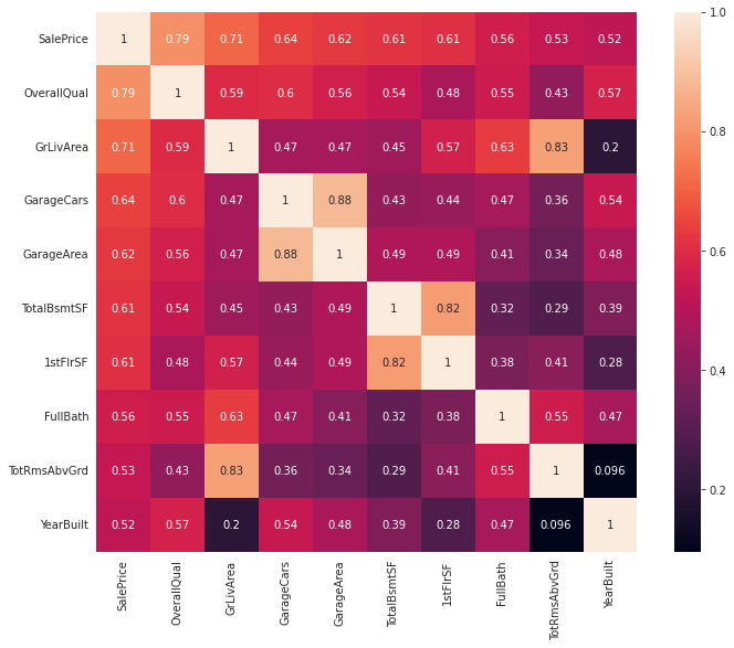
Quantitative Data Exploration Notes

We can now see quite clearly what variables relate to each other. Since we are only interested in the variables in relationship to saleprice, we can take a look at last row, or the last columm. remember, since the lighter colors are higher in value, listing the columns which output the lighter boxes means there’s a strong relationship between the variables. Oveall, we can observe four total categories.

notes: SF = square footage

Quality - overall quality, overall condition
Area dependant - Lot area, gros living area, basement area, garage area
date dependant -Year bulit, year remodeled
Amenities - number of baths, bedrooms, fireplaces, garage cars

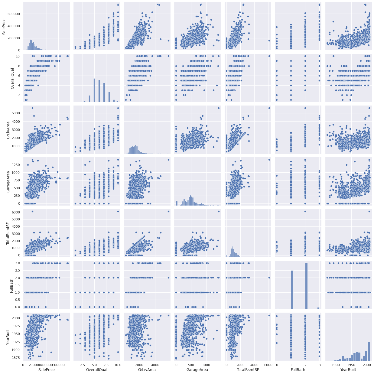
For the following, I’ll plot a scatter chart isolating these variables, and then see if there is a trend between these variables just in case we need to explore more for each of these trends.

Notes:

Garage Cars was removed due to redundancy with Garage Area

sns.set_theme(style="whitegrid")
sns.set()
cols = ['SalePrice', 'OverallQual', 'GrLivArea', 'GarageArea', 'TotalBsmtSF', 'FullBath', 'YearBuilt']
sns.pairplot(df_train[cols], size = 2.5)
plt.show();

png

Qualatative Data

With Qualatiative Data, it’s a bit more tricky to analyze, but there are some ways we can still perform it. Here’s list of variables that is avaiable to us.A simple idea is this. We can try to eliminate the two main numerical factors influencing the salesprice, which is the floor area. to help better isolate for the current analyzed variable. to do this:

Divide the sales price by the floor area, to get price per sqft.
Plot each variable with a boxplot.
Inspect each one and see if there is any correlation.

just as a reminder, here are the qualatiative featuers of our dataset.

print("\n ------ Qualatative data ---------\n")
print(qual_cols)

 ------ Qualatative data ---------

['MSZoning', 'Street', 'Alley', 'LotShape', 'LandContour', 'Utilities', 'LotConfig', 'LandSlope', 'Neighborhood', 'Condition1', 'Condition2', 'BldgType', 'HouseStyle', 'RoofStyle', 'RoofMatl', 'Exterior1st', 'Exterior2nd', 'MasVnrType', 'ExterQual', 'ExterCond', 'Foundation', 'BsmtQual', 'BsmtCond', 'BsmtExposure', 'BsmtFinType1', 'BsmtFinType2', 'Heating', 'HeatingQC', 'CentralAir', 'Electrical', 'KitchenQual', 'Functional', 'FireplaceQu', 'GarageType', 'GarageFinish', 'GarageQual', 'GarageCond', 'PavedDrive', 'PoolQC', 'Fence', 'MiscFeature', 'SaleType', 'SaleCondition']

Variable analysis

Lot Shaping such as: MSZoning, LotShape, LandContour, LotConfig, LandSlope have a low chance of influencing price, these are just not something that would influence price from a common sense standpoint.
Conditions such as ‘Condition1’, ‘ExterQual’ etc, is already categorized into the general condition, which is better since it is numeric.
Material & Anemities such as ‘MasVnrType’ or ‘CentralAir’ may influence the house price, however, these more influence the operational cost and have much less of an impact when compared to items such as sqft.

which really only leaves us with something like neighboorhood which we can consider adding in, as this is something many people consider when choosing a house. To say it simply, you can have a really big house, but if it’s in the middle of nowhere, then obviously the house price goes down. For now, each variable will be plotted with a boxplot and then compared to salesprice to see if I’m incorrect in my assumptions.

df_train['Price_per_sqft'] = df_train['SalePrice'] / df_train['GrLivArea'] 
df_train

	Id	MSSubClass	MSZoning	LotFrontage	LotArea	Street	Alley	LotShape	LandContour	Utilities	...	PoolQC	Fence	MiscFeature	MiscVal	MoSold	YrSold	SaleType	SaleCondition	SalePrice	Price_per_sqft
0	1	60	RL	65.0	8450	Pave	NaN	Reg	Lvl	AllPub	...	NaN	NaN	NaN	0	2	2008	WD	Normal	208500	121.929825
1	2	20	RL	80.0	9600	Pave	NaN	Reg	Lvl	AllPub	...	NaN	NaN	NaN	0	5	2007	WD	Normal	181500	143.819334
2	3	60	RL	68.0	11250	Pave	NaN	IR1	Lvl	AllPub	...	NaN	NaN	NaN	0	9	2008	WD	Normal	223500	125.139978
3	4	70	RL	60.0	9550	Pave	NaN	IR1	Lvl	AllPub	...	NaN	NaN	NaN	0	2	2006	WD	Abnorml	140000	81.537566
4	5	60	RL	84.0	14260	Pave	NaN	IR1	Lvl	AllPub	...	NaN	NaN	NaN	0	12	2008	WD	Normal	250000	113.739763
...	...	...	...	...	...	...	...	...	...	...	...	...	...	...	...	...	...	...	...	...	...
1455	1456	60	RL	62.0	7917	Pave	NaN	Reg	Lvl	AllPub	...	NaN	NaN	NaN	0	8	2007	WD	Normal	175000	106.253795
1456	1457	20	RL	85.0	13175	Pave	NaN	Reg	Lvl	AllPub	...	NaN	MnPrv	NaN	0	2	2010	WD	Normal	210000	101.302460
1457	1458	70	RL	66.0	9042	Pave	NaN	Reg	Lvl	AllPub	...	NaN	GdPrv	Shed	2500	5	2010	WD	Normal	266500	113.888889
1458	1459	20	RL	68.0	9717	Pave	NaN	Reg	Lvl	AllPub	...	NaN	NaN	NaN	0	4	2010	WD	Normal	142125	131.841373
1459	1460	20	RL	75.0	9937	Pave	NaN	Reg	Lvl	AllPub	...	NaN	NaN	NaN	0	6	2008	WD	Normal	147500	117.436306

1460 rows × 82 columns

# define that plots and sorts qual variable when compared to salesprice. 

def qual_var_calc(var):
    
    dep_var = 'SalePrice'
    df_var_sqft = df_train[[var , dep_var]]


    df_var_sqft_by_categ = df_var_sqft.groupby(var).mean()
    df_var_sqft_by_categ = df_var_sqft_by_categ.sort_values(by = dep_var, ascending = False)
    order_list = list(df_var_sqft_by_categ.index)

    plt.subplots(figsize=(9, 6))
    plt.title(str(var) + ' vs. SalePrice')
    plt.xticks(rotation=90)
    sns.boxplot(x=var, y=dep_var, data=df_var_sqft, order = order_list)

# for i in qual_cols:
#     qual_var_calc(i)

Filling in missing data.

Now that We’ve done some EDA to see some relationships with variables, it’s time to see what needs to be cleaned up in the data. This is important becauese data needs to be complete and rid of errors in order to get accurate results. Some things to keep in mind when cleaning data are:

Are the errors random, or do they have a pattern? what does this impact if I change it?

A good first step in cleaning up data is to find out the null, or missing values

total_null_values = df_train.isnull().sum().sort_values(ascending = False)
percent_null_values = (df_train.isnull().sum()/df_train.isnull().count()).sort_values(ascending = False)

total_null_values
percent_null_values
missing_data = pd.DataFrame()

missing_data['no. of missing values'] = total_null_values
missing_data['percent of missing values'] = percent_null_values

display(missing_data.head(30))

# delete columsn 
cols_to_delete = missing_data[missing_data['percent of missing values'] > 0].index


df_train = df_train.drop(columns = list(cols_to_delete))

print("\n ------ Columns with no missing data ---------\n")
df_train.columns

	no. of missing values	percent of missing values
PoolQC	1453	0.995205
MiscFeature	1406	0.963014
Alley	1369	0.937671
Fence	1179	0.807534
FireplaceQu	690	0.472603
LotFrontage	259	0.177397
GarageType	81	0.055479
GarageYrBlt	81	0.055479
GarageCond	81	0.055479
GarageQual	81	0.055479
GarageFinish	81	0.055479
BsmtFinType2	38	0.026027
BsmtExposure	38	0.026027
BsmtQual	37	0.025342
BsmtCond	37	0.025342
BsmtFinType1	37	0.025342
MasVnrType	8	0.005479
MasVnrArea	8	0.005479
Electrical	1	0.000685
Id	0	0.000000
Fireplaces	0	0.000000
Functional	0	0.000000
KitchenQual	0	0.000000
KitchenAbvGr	0	0.000000
BedroomAbvGr	0	0.000000
HalfBath	0	0.000000
FullBath	0	0.000000
BsmtHalfBath	0	0.000000
TotRmsAbvGrd	0	0.000000
GarageCars	0	0.000000

 ------ Columns with no missing data ---------






Index(['Id', 'MSSubClass', 'MSZoning', 'LotArea', 'Street', 'LotShape',
       'LandContour', 'Utilities', 'LotConfig', 'LandSlope', 'Neighborhood',
       'Condition1', 'Condition2', 'BldgType', 'HouseStyle', 'OverallQual',
       'OverallCond', 'YearBuilt', 'YearRemodAdd', 'RoofStyle', 'RoofMatl',
       'Exterior1st', 'Exterior2nd', 'ExterQual', 'ExterCond', 'Foundation',
       'BsmtFinSF1', 'BsmtFinSF2', 'BsmtUnfSF', 'TotalBsmtSF', 'Heating',
       'HeatingQC', 'CentralAir', '1stFlrSF', '2ndFlrSF', 'LowQualFinSF',
       'GrLivArea', 'BsmtFullBath', 'BsmtHalfBath', 'FullBath', 'HalfBath',
       'BedroomAbvGr', 'KitchenAbvGr', 'KitchenQual', 'TotRmsAbvGrd',
       'Functional', 'Fireplaces', 'GarageCars', 'GarageArea', 'PavedDrive',
       'WoodDeckSF', 'OpenPorchSF', 'EnclosedPorch', '3SsnPorch',
       'ScreenPorch', 'PoolArea', 'MiscVal', 'MoSold', 'YrSold', 'SaleType',
       'SaleCondition', 'SalePrice', 'Price_per_sqft'],
      dtype='object')

So the above table tells us what variables have missing values. Since in this particular case, there are not a lot of missing data, therefore we could consider to look at them one by one and then determine based on “feel” if they contribute to the price of the house. If I had to arbituraly decide what is a threshold that a variable is just straight up unsusable, I would say that it’s above 20% missing. This means that variables such as PoolQC, MiscFeature and Alley might be just straight up irrelevant to determining the house prices, so we can go ahead and delete those.

In this case, all the variables do not seem crutial to determining the price of the house.

Checking Sales Price

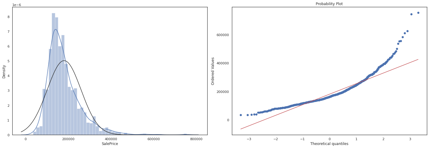
Now that we’ve done some EDA, it’s time to finally analyze our dependant variable: Sales Price there are two particular things we are looking out for.

Histogram - Kurtosis and skewness. Normal probability plot - Data distribution should closely follow the diagonal that represents the normal distribution.

Question what is skewness and kurtosis? and why does it matter?

Answer

Skewness measures the asymmetry of a distribution. It indicates whether the data is skewed to the left (negative skewness) or to the right (positive skewness). A perfectly symmetrical distribution has a skewness of zero.

Positive skewness: If the distribution has a longer tail on the right side and most of the data is concentrated on the left side, it is positively skewed.
Negative skewness: If the distribution has a longer tail on the left side and most of the data is concentrated on the right side, it is negatively skewed.

Kurtosis measures the peakedness or flatness of a distribution. It provides information about the tails of the distribution and whether it has outliers compared to a normal distribution. A normal distribution has a kurtosis of 3 (referred to as mesokurtic).

Leptokurtic distribution: If the distribution has a higher peak and heavier tails compared to a normal distribution, it is leptokurtic (kurtosis > 3).
Platykurtic distribution: If the distribution has a flatter peak and lighter tails compared to a normal distribution, it is platykurtic (kurtosis < 3).

Certain machine learning algorithms assume that the data follows specific distributions, such as normality. Skewness and kurtosis provide insights into the departure from these assumptions. If the data violates these assumptions, it may affect the model’s performance or the validity of certain statistical tests used in the modeling process.

sns.set_theme(style = 'white')
fig = plt.figure(figsize=(20,7))

fig1 = fig.add_subplot(121)

sns.distplot(df_train['SalePrice'], fit= norm)
fig2 = fig.add_subplot(122)
res = stats.probplot(df_train['SalePrice'], plot=plt)

plt.tight_layout()
plt.show()

png

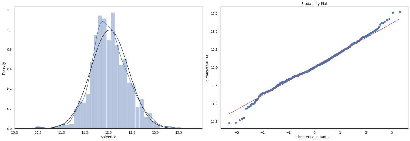
#log1p which applies log(1+x) to all elements of the column and normalizes the data. 

df_train['SalePrice'] = np.log1p(df_train['SalePrice'])

sns.set_theme(style = 'white')
fig = plt.figure(figsize=(20,7))

fig1 = fig.add_subplot(121)

sns.distplot(df_train['SalePrice'], fit= norm)
fig2 = fig.add_subplot(122)
res = stats.probplot(df_train['SalePrice'], plot=plt)

plt.tight_layout()
plt.show()

png

Machine Learning

Once we’ve done some EDA, it’s time to see if any ML algo can help us predict a house price. The general outline for this section is to:

Create a Dataset which uses previously explored variables which have the highest correlation with sales price.
Run different models and predict house prices
Compare which housing prices are most accuratly predicted using MAE, and RMSE to see if the algorithm is any good

Constructing Dataset for machine learning

# copy and keep most important variables 

df_train_ml = df_train.copy()
feat_var = ['SalePrice', 'OverallQual', 'GrLivArea', 'GarageArea', 'TotalBsmtSF', 'FullBath', 'YearBuilt','Neighborhood']
df_train_ml = df_train_ml[feat_var]

# check for mull values

print('\n -------- Null values -----------\n')
print(df_train_ml.isnull().sum())

# factorize neighboorhoods (convert to numeric)

arr, ind = df_train_ml['Neighborhood'].factorize()
df_train_ml['Neighborhood'] = arr

 -------- Null values -----------

SalePrice       0
OverallQual     0
GrLivArea       0
GarageArea      0
TotalBsmtSF     0
FullBath        0
YearBuilt       0
Neighborhood    0
dtype: int64

Training a ML model (notes)

For this, we will use python’s scikit learn to build a machine learning model. To start, I just want to see what the machine learning predicts with a basic linear regession model. But before we get into that, I want to explore some basic machine learning concepts.

The goal of machine learning is to enable computers to automatically learn from data and improve their performance on a specific task over time.

Supervised Learning:

Supervised learning is a type of machine learning where the algorithm is trained on labeled data. Labeled data refers to data that has both input features and corresponding target labels or outcomes. The goal of supervised learning is to learn a mapping function that can predict the correct output or label for new, unseen input data. The algorithm learns from the labeled examples provided during training and then generalizes to make predictions on new, unlabeled data. Supervised learning can be further classified into two main categories: regression and classification. In regression, the goal is to predict a continuous numerical value, while in classification, the goal is to predict a class or category.

Unsupervised Learning:

Unsupervised learning, on the other hand, involves training an algorithm on unlabeled data. Unlabeled data refers to data that does not have any predefined target labels or outcomes. The goal of unsupervised learning is to discover patterns, structures, or relationships within the data. The algorithm learns from the inherent structure or statistical properties of the data and identifies similarities, clusters, or other patterns without any explicit guidance. Unsupervised learning algorithms are useful for tasks such as clustering, dimensionality reduction, and anomaly detection.

For supervised learning, there are two types:

Regression:

Regression is a type of supervised learning where the goal is to predict a continuous numerical value as the output. In regression, the target variable is a continuous variable, meaning it can take any value within a range. The task is to learn a mapping function from the input features to the continuous output variable. For example, predicting house prices, stock prices, or the temperature can be framed as regression problems. The algorithm learns from labeled examples where both the input features and their corresponding continuous output values are known. During training, the regression model tries to find the best fit or approximation to the underlying relationship between the input variables and the continuous target variable.

Classification:

Classification, on the other hand, is a type of supervised learning where the goal is to assign input data points into predefined categories or classes. In classification, the target variable is discrete and represents specific classes or categories. The task is to learn a mapping function that can accurately classify new, unseen data points into one of the predefined classes. For example, email spam detection, sentiment analysis, or image classification tasks are all classification problems. During training, the classification algorithm learns from labeled examples where the input features are known, and each example is associated with a class or category label.

for predicting prices, supervised learning with regression models will be used

Results Discussion:

As you can see, we’re not really off to a great start. This is because the model is predicting a house price that is off around 30,000 dollars according to the MAE, and 126,000 dollars accourding to the RMSE.
This means that if you’re house is worth at 500,000 dollars, it could be worth anywhere between 530,000 and 470,000 dollars. This is okay but let’s see if we can get the number any lower than this number. We have a lot of ways to do that, so let me explain to myself first.

Question: Why is the RMSE so much higher than the MAE?
Answer: this is because the math behind how they are calculated. In general, the RMSE is much more sensetive to outliers, which means that you might get a much larger number.

for reference: check out this page on how MAE and RMSE are calcualted

What can I blame for the bad performance:

The ML Algorithm sucks, or it’s just not good in this case

Problem: This algorithm is not the right one for the job.
Solution: Try out different models which use different computation methods and see which one fits the best.

The training data was not representative of the whole dataset, aka, trained on the wrong data?

Problem: Basically, let’s say that I have like my data had like 5 houses with a floor area of 10,000 sqft but only cost 2 dollars. Since my model would be trained on that, it would cause some problems
Solution: Change the train test split and re-elvaluate.

The selected features are bad.

Problem: well, I have too many features, which is causing overfitting. (more on this later)
Solution: try out different combinations of features

notes on model-cross validation

Cross-validation is an essential technique in machine learning for model evaluation and selection. It involves dividing the available dataset into multiple subsets or folds to assess the model’s performance on unseen data. The main reasons why cross-validation is important are:

Robust Performance Estimation: Cross-validation provides a more reliable estimate of the model’s performance by using multiple evaluations on different subsets of the data. It helps to mitigate the impact of random variations in the dataset and provides a more robust estimate of the model’s generalization ability.
Overfitting Detection: Cross-validation helps in identifying whether a model is overfitting the training data. Overfitting occurs when a model learns the specific patterns or noise in the training data to the extent that it performs poorly on new, unseen data. By evaluating the model on multiple folds, cross-validation can highlight instances where the model’s performance degrades due to overfitting.
Hyperparameter Tuning: Machine learning models often have hyperparameters, which are settings or configurations that are not learned from the data but need to be set by the user. Cross-validation helps in finding the optimal values for these hyperparameters by repeatedly training and evaluating the model on different subsets of the data. It allows the selection of hyperparameter values that yield the best generalization performance.

K-fold cross-validation is a common cross-validation technique. It involves dividing the dataset into K equally sized folds or subsets. The cross-validation process then iterates K times, each time using a different fold as the validation set while the remaining folds are used for training. The steps of k-fold cross-validation are as follows:

The dataset is randomly shuffled to ensure that the data is distributed evenly across folds.
The dataset is divided into K equal-sized folds.
The training and evaluation process is performed K times. In each iteration:
- One fold is held out as the validation set.
- The model is trained on the remaining K-1 folds.
- The model’s performance is evaluated on the validation set using an evaluation metric (e.g., accuracy, MAE, RMSE).
- The performance results from the K iterations are averaged to obtain an overall performance estimate for the model.

K-fold cross-validation helps in achieving a better estimate of the model’s performance by reducing the variance in performance estimation compared to a single train-test split. It allows for more thorough evaluation and comparison of different models or hyperparameter settings.

Typical values for K are 5 or 10, but it can vary depending on the size of the dataset and the computational resources available. Other variations of cross-validation, such as stratified k-fold or leave-one-out cross-validation, can also be used based on the specific requirements of the problem at hand.

# importing and testing different ML models
from sklearn.tree import DecisionTreeRegressor
from sklearn import linear_model 
from sklearn.neighbors import NearestCentroid
from sklearn import svm
from sklearn.naive_bayes import GaussianNB
from sklearn.preprocessing import StandardScaler 


# create a function that test models with different ML models 

ML_alog = [DecisionTreeRegressor(),
           linear_model.LinearRegression(),
           linear_model.Ridge(alpha=.5),
           linear_model.BayesianRidge(),
          NearestCentroid(),
          svm.SVR()] 

from sklearn.model_selection import cross_val_score
from sklearn.model_selection import KFold

def ml_model_cross_val(features,model):

    X = df_train_ml[features]
    y = df_train_ml['SalePrice']

    #cross validation 
    k_folds = KFold(n_splits = 5)
    scores = cross_val_score(model, X, y, cv = k_folds)
    return scores

algo_scores = {}
feats_all = ['OverallQual', 'GrLivArea', 'GarageArea', 'TotalBsmtSF', 'FullBath', 'YearBuilt','Neighborhood']

for mod in ML_alog:

    score = ml_model_cross_val(feats_all,mod)
    algo_scores[str(mod)] = score.mean()
    

print('\n -------- Model cross validation scores -----------\n')
algo_scores

 -------- Model cross validation scores -----------

{'DecisionTreeRegressor()': 0.6753158731560609,
 'LinearRegression()': 0.7989489108161099,
 'Ridge(alpha=0.5)': 0.7989492488152841,
 'BayesianRidge()': 0.7989073632186516,
 'NearestCentroid()': nan,
 'SVR()': 0.7736577239479618}

As we can see, the best performing model is the ‘DecisionTreeRegressor’. We will be using this from now on. The next step is to make a function that tests different combinations of features, for this, every combination will be tested to see which one produces the lowest MAE and RMSE.

# creating a function that can adjust for different ML models and features
# returns the MAE and RMSE

def ml_model_selection(features,model):

    X = df_train_ml[features]
    y = df_train_ml['SalePrice']

    # split model 
    train_X, val_X, train_y, val_y = train_test_split(X, y, random_state = 0)


    # fit model (train the model to predict house prices)
    house_pred_model = model
    house_pred_model.fit(train_X, train_y)
    val_predictions = house_pred_model.predict(val_X)

    # make dataframe to compare predicted and actual values 
    predictions_df = pd.DataFrame() 
    predictions_df['Predictions'] = val_predictions
    predictions_df = predictions_df.set_index(keys = val_y.index)
    predictions_df['Actual'] = val_y

    predictions_df

    # create df to refelct original prices 
    og_predictions_price_df = np.expm1(predictions_df)
    og_predictions_price_df


    # calculate MAE and RSME to check model performance 
    price_MAE = mean_absolute_error(og_predictions_price_df['Actual'], og_predictions_price_df['Predictions'])
    price_RMSE = mean_squared_error(og_predictions_price_df['Actual'], og_predictions_price_df['Predictions'], squared = False)


    return price_MAE, price_RMSE

### create function to get every combinations of features. 

import itertools

feat_combos = [] 

feats_all = ['OverallQual', 'GrLivArea', 'GarageArea', 'TotalBsmtSF', 'FullBath', 'YearBuilt','Neighborhood']
for L in range(len(feats_all) + 1):
    for subset in itertools.combinations(feats_all, L):
        feat_combos.append(list(subset))
        
feat_combos = feat_combos[1:]    

feature_names = [] 
comb_mae = [] 
comb_rsme = [] 

for feat_c in feat_combos: 
    
    mae, rsme = ml_model_selection(feat_c, DecisionTreeRegressor())
    feature_names.append(feat_c)
    comb_mae.append(mae)
    comb_rsme.append(rsme)
    
d = {'feature_names':feature_names, 'comb_mae':  comb_mae,'comb_rsme':comb_rsme}
feat_combo_df = pd.DataFrame(data = d)


feat_combo_df['tot_err'] = feat_combo_df['comb_mae'] + feat_combo_df['comb_rsme']

print('\n -------- features with lowest MAE and RSME -----------\n')
print(feat_combo_df.sort_values(by = 'tot_err').iloc[0]['feature_names'])

print('\n')
display(feat_combo_df.sort_values(by = 'tot_err').head(1))

 -------- features with lowest MAE and RSME -----------

['OverallQual', 'GrLivArea', 'TotalBsmtSF', 'FullBath', 'YearBuilt', 'Neighborhood']

	feature_names	comb_mae	comb_rsme	tot_err
123	[OverallQual, GrLivArea, TotalBsmtSF, FullBath...	24870.073404	36856.824607	61726.898011

df_train2 = pd.read_csv('../input/house-prices-advanced-regression-techniques/train.csv')
df_train2['SalePrice'].mean()

180921.19589041095

Refined Model Discussion

We’ve created a better model than the intial linear regression model. Although the MAE increased very slightly, the RMSE decreased by a significant amount, which shows the improvement be refinding the model and the features.

Given that the average house price is around 181,000 dollars, given the error between the refined version of the model, we would be about a 13% error range, and about 20% for the RMSE. Since RMSE is more sensetive to outliers, that may be something to look into next time. Now time to apply it to a testing model and re-evaluate. We will simply just copy the last portion of the code and then replace the training with the testing model

Test Model Input

using the refined variables:

Features: [‘OverallQual’, ‘GrLivArea’, ‘TotalBsmtSF’, ‘YearBuilt’, ‘Neighborhood’]
Model Decision Tree Regressor

# copy and keep most important variables 

df_test_ml = df_test.copy()
feat_var_test = ['OverallQual', 'GrLivArea', 'TotalBsmtSF', 'YearBuilt', 'Neighborhood']
df_test_ml = df_test_ml[feat_var_test]

# check for mull values

print('\n -------- Null values -----------\n')
print(df_test_ml.isnull().sum())

# factorize neighboorhoods (convert to numeric)

arr, ind = df_test_ml['Neighborhood'].factorize()
df_test_ml['Neighborhood'] = arr

df_test_ml = df_test_ml.dropna()

print('\n -------- Null values check -----------\n')
print(df_test_ml.isnull().sum())

 -------- Null values -----------

OverallQual     0
GrLivArea       0
TotalBsmtSF     1
YearBuilt       0
Neighborhood    0
dtype: int64

 -------- Null values check -----------

OverallQual     0
GrLivArea       0
TotalBsmtSF     0
YearBuilt       0
Neighborhood    0
dtype: int64

# set up training and test datasets 

train_X = df_train_ml[feat_var_test]
train_y = df_train_ml['SalePrice']
test_X = df_test_ml[feat_var_test]

house_pred_model = DecisionTreeRegressor()
house_pred_model.fit(train_X, train_y)
val_predictions = house_pred_model.predict(test_X)

# make dataframe to compare predicted and actual values 
predictions_df =  test_X.copy()
predictions_df['Predictions'] = np.expm1(val_predictions)

predictions_df.head()

	OverallQual	GrLivArea	TotalBsmtSF	YearBuilt	Neighborhood	Predictions
0	5	896	882.0	1961	0	144000.0
1	6	1329	1329.0	1958	0	140000.0
2	5	1629	928.0	1997	1	131500.0
3	6	1604	926.0	1998	1	200500.0
4	8	1280	1280.0	1992	2	245500.0

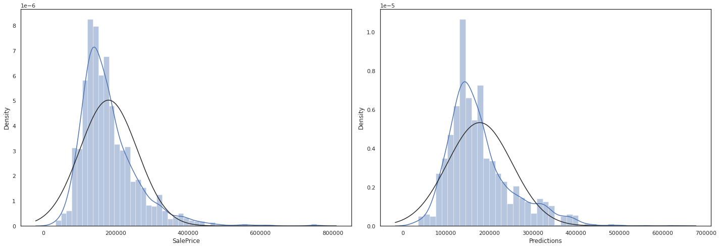
Final check

Since we have no way to check if our predictions are right, I can at least take a look at the distribution which seems okay

sns.set_theme(style = 'white')
fig = plt.figure(figsize=(20,7))

fig1 = fig.add_subplot(121)
sns.distplot(np.expm1(df_train['SalePrice']), fit= norm)

fig2 = fig.add_subplot(122)
sns.distplot(predictions_df['Predictions'], fit= norm)

plt.tight_layout()
plt.show()

png

Conclusion

This has been a machine learning project intended to get me started on machine learning basics. In no way is this a super advance and comprehensive solution. This project however, is designed to get me more familiar with the concepts of data exploration, feature engineering, and using basic machine learning models to predict values.

Strong points:

Quite robust EDA section, which explored all of the quantative data to find correlation between featuers and target variables
explored many different models to see which one was best suited to predict house prices
different combinations of features were tested.

Improvements:

explore how to incorperate more ways to include categoical data.
for ML models, it would be good to understand at least the basics of the black box, it can help me know what models to use faster.
maybe also try using machine learning for the feature selection.
include more statical methods to reinforce findings. For instance, to see if the neighborhoods really have a strong effect on house prices (maybe ANOVA testing)
use deep neural networks such as tensorflow to see if a more accurate prediction can be made.

References

https://www.kaggle.com/learn/intro-to-machine-learning https://www.kaggle.com/code/mgmarques/houses-prices-complete-solution
https://www.kaggle.com/code/pmarcelino/comprehensive-data-exploration-with-python
https://towardsdatascience.com/7-of-the-most-commonly-used-regression-algorithms-and-how-to-choose-the-right-one-fc3c8890f9e3

COMPREHENSIVE DATA EXPLORATION WITH PYTHON’ written by Pedro Marcelino
MARCELO MARQUES, Houses Prices - Complete Solution

Rayen Feng

Check out my Blog!