Anime Recomendations systems

The data science team at myanimelist.net wants to improve their site and create a recommendation system using machine learning techniques to recommend animes to users. Information is webscraped to construct an anime database, then two recommendation systems are built using a content filtering system and a collaborative filtering system.

A recommender using content-based filtering was constructed using the features of the anime, such as genre, and description. The content-based recommendation system is proficient at detecting the sequels of the anime based on their plot lines, however, it led to a dry and repetitive user experience as the recommended content is too similar. Next, user information was gathered and a recommender using the collaborative filtering was built. Five different algorithms were cross validated, of which, the SVD algorithm performed the best and was implemented into the system. The results were investigated using a sample user, and the results from this method were accurate in their predictions.

Given the already robust database that myanimelist.net has, both approaches would have no restrictions if they are implemented, although a collaborative filtering approach seems to produce the more accurate results and is the favoured approach to use. However, based on the results of this study, a hybrid approach may need to be used to take the strengths of each method.

Building Concent reccomendation system

The first section of this report will focus on building a content-based recommender system. A content filtering recommendation system works by analyzing the content of the items and using that information to identify other items that are similar in terms of their content. In this case, this could be features such as the plot of the series, similar genres, characters, etc.

The analysis for the content recommendation systems will be as follows:

1. Data on the 10,000 anime will be scraped and cleaned. This notebook uses the results from the webscraping code, which can be found in other notebooks
2. Data exploration and feature engineering will be performed to find outliers, trends, and correlations.
3. A content recommendation system will be built by finding similar shows in specific categories.

import numpy as np
from bs4 import BeautifulSoup
import requests
import re
import requests
import lxml.html as lh
import pandas as pd
import pickle
import os 
import scipy.stats as stats
import seaborn as sns
import matplotlib.pyplot as plt

pd.options.mode.chained_assignment = None  # default='warn'

from sklearn.feature_extraction.text import CountVectorizer, TfidfVectorizer
from sklearn.cluster import KMeans
from sklearn.metrics.pairwise import cosine_similarity, linear_kernel
from sklearn.decomposition import PCA

EDA: Exploring the data

The purpose of this segment is to get familiar with the data. This is to see if the human eye can detect any outliers and manually remove them. Also, this is a good chance to do some feature engineering and see if any of the features are a strong indicator of score.

Some things to explore might be:

1. Are there any outliers in each of the categories:
   • are there anime with more than x studios, producers, demographics
2. If the featuers are categorical, What are the categories of each feature and how many?

Some questions might include:

1. is studio correlated with score?
2. is time of production correlated with score?
3. does genre have a correlation with score?
4. can I analyze the top 100 anime of all time and see what common trends I see.
5. average studio production rating.

Another key process is feature engineering, which is the process of selecting the most relevant features, or variables for a model. During this process, it is also worth investigating if any of the features would be a key predictor in determining the public rating. Below, the outputs printed shows the percentage of missing values for each of the features in the anime details dataframe. To reduce the number of variables, features can be eliminated based on their lack of data and whether or not they duplicate information from another column. For instance, the column “aired_start” which is the start broadcast date, is reliable, while its counterpart “aired_end” can be removed as it has too many missing values. It can also be observed that combining the columns from “genre” and “genres” into “genres_overall” did have a significant effect because the null values in the column were reduced to 7%. Although ‘genres_overall’ has the majority of the records filled, “themes_overall” and “demographics_overall” still have many missing values. Since themes and demographics has somewhat of an overlap with the information provided by genres, they will be removed due to the data being relatively unreliable.

top_anime_all_table = pd.read_csv('/Users/rayenfeng/Documents/code/anime_rec_project/data_sources_pickle/all_anime_directory.csv')
#top_anime_all_table.head()

# import clean frame 
with open('/Users/rayenfeng/Documents/code/anime_rec_project/data_sources_pickle/all_anime_details_frame_no_nan_cvas.pkl', 'rb') as f:
    all_anime_details_frame_no_nan_cvas = pickle.load(f)

with open('/Users/rayenfeng/Documents/code/anime_rec_project/data_sources_pickle/anime_info_frame_cleaned_main.pkl', 'rb') as f:
    anime_info_frame_cleaned = pickle.load(f)

# percentage of missing values per column, use columns with less missing for more data reliability. 

print("Percent Missing")
anime_info_frame_cleaned.isna().sum() * 100/ len(anime_info_frame_cleaned)

Percent Missing





English                 42.77
Type                     0.00
Episodes                 0.00
Status                   0.00
aired_start              1.99
aired_end               44.28
premiered               61.09
broadcast_weekday       74.20
broadcast_daytime       74.72
producers               35.44
studios                 12.27
source                   0.00
genres_multi            30.69
genres_singular         76.99
genres_overall           7.68
themes_singular         60.54
themes_multi            70.29
themes_overall          30.83
demographic_singular    64.40
demographics_multi      99.21
demographics_overall    63.61
duration_in_min          0.08
public_score_rating      0.00
popularity               0.00
Favorites                0.00
Completed                0.00
On-Hold                  0.00
Dropped                  0.00
Plan to Watch            0.00
Total                    0.00
dtype: float64

Score distribution

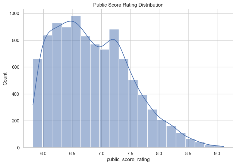
A key feature is “public_score_rating”, which is the average score that users give a certain anime. This can be plotted on a histogram to see the rating distribution. The below figure shows the rating score distribution and as expected, the distribution is skewed to the right, with the average score being about 6.9. It is important to note that this data was scraped in order of user ranking, therefore, the expected mean is slightly lower than what is shown.

plt.subplots(figsize=(9,6))
sns.set_theme(style="whitegrid")
sns.histplot(data=anime_info_frame_cleaned, x="public_score_rating", bins = 20, kde = True)
plt.title('Public Score Rating Distribution')
anime_info_frame_cleaned.describe().round(1)

	Episodes	aired_start	aired_end	duration_in_min	public_score_rating	popularity	Favorites	Completed	On-Hold	Dropped	Plan to Watch	Total
count	10000.0	9801	5572	9992.0	10000.0	10000.0	10000.0	10000.0	10000.0	10000.0	10000.0	10000.0
mean	14.4	2008-12-17 17:05:49.311294720	2008-12-19 11:16:03.962670336	29.0	6.9	6324.2	982.0	53621.1	2119.5	2567.1	19067.7	82313.8
min	1.0	1929-10-14 00:00:00	1962-02-25 00:00:00	0.2	5.8	1.0	0.0	0.0	0.0	1.0	13.0	180.0
25%	1.0	2003-08-01 00:00:00	2003-09-25 00:00:00	13.0	6.3	2610.5	3.0	1054.8	55.0	92.0	878.0	2452.8
50%	4.0	2012-04-07 00:00:00	2012-01-26 00:00:00	24.0	6.8	5624.5	17.0	5472.5	219.0	221.5	3588.0	10733.0
75%	13.0	2017-10-06 00:00:00	2017-09-26 06:00:00	26.0	7.3	9680.2	148.0	32157.0	1110.2	1184.0	15501.8	55669.0
max	3057.0	2022-12-01 00:00:00	2023-01-08 00:00:00	168.0	9.1	18239.0	210883.0	3133727.0	168119.0	203501.0	586370.0	3580542.0
std	49.2	NaN	NaN	27.3	0.7	4332.2	6279.9	167132.2	6788.4	7588.8	40923.0	224824.1

Date vs score

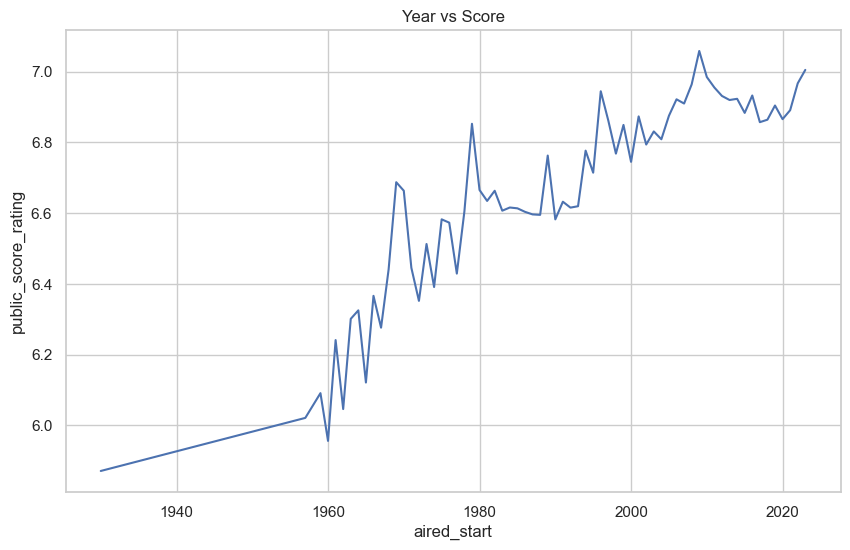
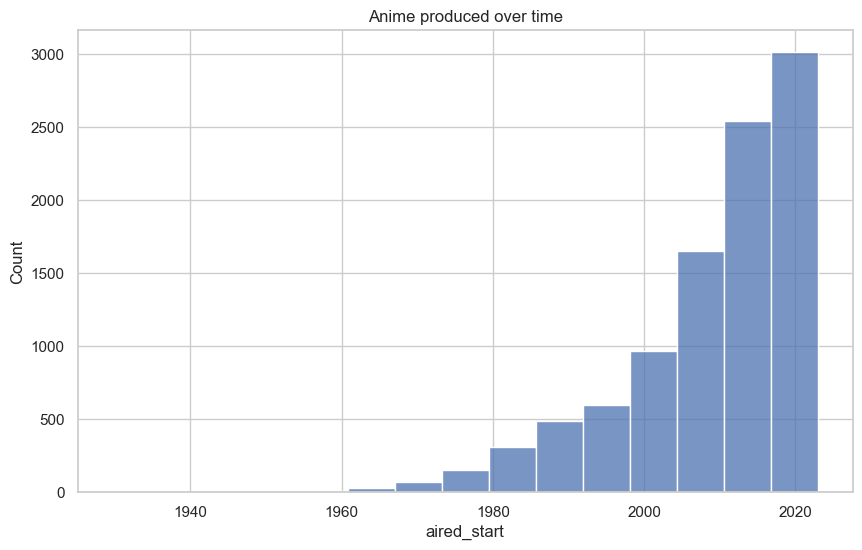
Another feature is the air date, which is the date which an anime started it’s broadcast. Figure 8 is a plot showing the average anime score in each year. As shown in the graph, it can be seen that the average anime rating seems to increase over time, especially starting from 1970. This is most likely because over the years, the production quality advanced with available technology. This along with anime being more popular in recent times may be a factor for the increase in score. This is shown by Figure 9, where the number of anime produced every year increases.

# rating by year 

info_by_year = anime_info_frame_cleaned.groupby(pd.Grouper(key='aired_start', axis=0, freq='Y'))['public_score_rating'].mean()
plt.subplots(figsize=(10,6))
sns.set_theme(style="whitegrid")
plt.title('Year vs Score')
sns.lineplot(data=info_by_year)

plt.show()

plt.subplots(figsize=(10,6))
plt.title('Anime produced over time')
sns.histplot(data=anime_info_frame_cleaned, x="aired_start", bins = 15)

<Axes: title={'center': 'Anime produced over time'}, xlabel='aired_start', ylabel='Count'>

# anime produced in 1929 seems to be an outlier, this is highlighted
anime_info_frame_cleaned[anime_info_frame_cleaned['aired_start'] == anime_info_frame_cleaned['aired_start'].min()]

	English	Type	Episodes	Status	aired_start	aired_end	premiered	broadcast_weekday	broadcast_daytime	producers	...	demographics_overall	duration_in_min	public_score_rating	popularity	Favorites	Completed	On-Hold	Dropped	Plan to Watch	Total
5875	The Stolen Lump	Movie	1	Finished Airing	1929-10-14	NaT	NaN	NaN	NaT	NaN	...	NaN	10.0	5.871	8952	2	2581	18	75	448	3177

1 rows × 30 columns

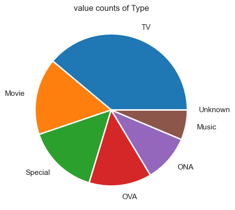
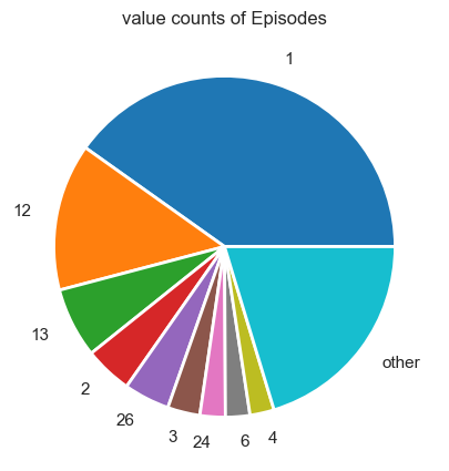
Data information on Episode Number and Type

def plot_pie_value_counts(series, sep_num):

    val_counts = series.value_counts()#.sort_values(ascending = False)
    first_sec = val_counts[:sep_num]
    other_sec = val_counts[sep_num:].sum()
    
    
    if other_sec > 0: 

        first_sec['other'] = other_sec

    plt.subplots(figsize=(6, 5))
    colors = sns.color_palette('tab10')
    plt.pie(first_sec,
            labels=first_sec.index,
            labeldistance=1.15,
            wedgeprops = { 'linewidth' : 2, 'edgecolor' : 'white'},
           colors = colors,)
    plt.title('value counts of ' + str(series.name))
    plt.show()

plot_pie_value_counts(anime_info_frame_cleaned['Type'], 7) 

plot_pie_value_counts(anime_info_frame_cleaned['Episodes'], 9)

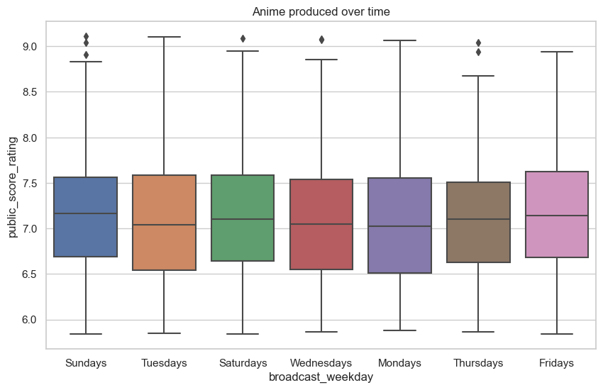
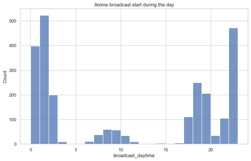
Aired time and weekday vs score

Another feature to investigate is the effect of broadcast time on the user score. Below is a boxplot that shows the average user score by weekday, while the following plot is a distribution of the number of shows that are broadcast during the day. It can be seen that the weekday does not make a significant difference in determining the score, however, it does seem that there are popular times to broadcast anime. As expected, there is a strong correlation with broadcast time with the school schedule, with most shows start broadcasting when students come home from school or stay up late into the night.

plt.subplots(figsize=(10,6))
plt.title('Anime produced over time')
sns.boxplot(data = anime_info_frame_cleaned, x= 'broadcast_weekday', y="public_score_rating") #, order=my_order)

#data=info_by_year, x = info_by_year.index,  y="public_score_rating")

<Axes: title={'center': 'Anime produced over time'}, xlabel='broadcast_weekday', ylabel='public_score_rating'>

hour_counts = anime_info_frame_cleaned['broadcast_daytime'].apply(lambda x: x.hour)

plt.subplots(figsize=(10,6))
plt.title('Anime broadcast start during the day')
sns.histplot(data=hour_counts, bins = 23)

<Axes: title={'center': 'Anime broadcast start during the day'}, xlabel='broadcast_daytime', ylabel='Count'>

# print(anime_info_frame_cleaned['studios'].dropna().apply(lambda y: len(y)).value_counts())
# print(anime_info_frame_cleaned['producers'].dropna().apply(lambda y: len(y)).value_counts())

# get list of anime with studios greater than 3 
len_of_studios = anime_info_frame_cleaned['studios'].dropna().apply(lambda y: len(y))
len_greater_studio = list(len_of_studios[len_of_studios > 3].index)
anime_info_frame_cleaned[anime_info_frame_cleaned['studios'].index.isin(len_greater_studio)]

	English	Type	Episodes	Status	aired_start	aired_end	premiered	broadcast_weekday	broadcast_daytime	producers	...	demographics_overall	duration_in_min	public_score_rating	popularity	Favorites	Completed	On-Hold	Dropped	Plan to Watch	Total
10178	NaN	Special	4	Finished Airing	2011-01-07	2013-03-24	NaN	NaN	NaT	[NHK]	...	[Josei]	25.0	7.371	4292	51	7407	886	507	10460	20787
42161	Pokétoon	ONA	8	Finished Airing	2020-06-04	2021-12-28	NaN	NaN	NaT	[Nintendo, Creatures Inc.]	...	[Kids]	8.0	7.351	7228	14	1732	682	247	1443	5779
28149	Japan Anima(tor)'s Exhibition	ONA	35	Finished Airing	2014-11-07	2015-10-09	NaN	NaN	NaT	[Dwango]	...	NaN	8.0	7.341	3198	123	12289	4178	1963	15517	38424
49357	Star Wars: Visions	ONA	9	Finished Airing	2021-09-22	NaT	NaN	NaN	NaT	[Twin Engine]	...	NaN	15.0	7.131	2122	379	46872	2900	2486	20000	78538
6867	Halo Legends	ONA	8	Finished Airing	2009-11-07	2010-02-16	NaN	NaN	NaT	[Casio Entertainment]	...	NaN	14.0	6.991	3154	192	28256	699	895	8662	39534
4094	Batman: Gotham Knight	OVA	6	Finished Airing	2008-07-08	NaT	NaN	NaN	NaT	[Cyclone Graphics]	...	NaN	12.0	6.941	3749	62	21344	250	325	5776	28174
2832	NaN	Special	15	Finished Airing	2007-06-07	2007-06-27	NaN	NaN	NaT	NaN	...	NaN	1.0	6.721	4201	9	13809	446	277	6981	21996
38022	Monster Strike the Animation	ONA	63	Finished Airing	2018-07-08	2019-12-31	NaN	NaN	NaT	[XFLAG]	...	NaN	10.0	6.681	7681	8	863	239	349	2844	5042
37290	Animation × Paralympic: Who Is Your Hero?	Special	15	Finished Airing	2017-11-10	2022-08-22	NaN	NaN	NaT	[NHK, NHK Enterprises]	...	NaN	5.0	6.481	11999	2	146	100	128	392	1043

9 rows × 30 columns

Genre, Theme and Demographic vs Score?

themes_overall_s_1 = anime_info_frame_cleaned['themes_overall'].dropna()
themes_overall_df_1 = pd.DataFrame(item for item in themes_overall_s_1).set_index(themes_overall_s_1.index)

demographics_overall_s_1 = anime_info_frame_cleaned['demographics_overall'].dropna()
demographics_overall_df_1 = pd.DataFrame(item for item in demographics_overall_s_1).set_index(demographics_overall_s_1.index)

genres_overall_s_1 = anime_info_frame_cleaned['genres_overall'].dropna()
genres_overall_df_1 = pd.DataFrame(item for item in genres_overall_s_1).set_index(genres_overall_s_1.index)

print('\n*********** Themes value counts ***********\n')
print(pd.Series(themes_overall_df_1.values.flatten()).value_counts())
print('\n*********** demographics value counts ***********\n')
print(pd.Series(demographics_overall_df_1.values.flatten()).value_counts())
print('\n*********** Genres value counts ***********\n')
print(pd.Series(genres_overall_df_1.values.flatten()).value_counts())

*********** Themes value counts ***********

School               1410
Music                1024
Mecha                 855
Historical            737
Military              489
Super Power           444
Mythology             387
Martial Arts          362
Space                 355
Adult Cast            341
Parody                340
Harem                 320
Psychological         297
Isekai                217
Detective             213
Team Sports           197
Mahou Shoujo          197
Idols (Female)        196
Gag Humor             183
Strategy Game         182
CGDCT                 176
Iyashikei             173
Samurai               143
Gore                  123
Vampire               120
Anthropomorphic       114
Workplace             105
Time Travel           102
Video Game             98
Idols (Male)           86
Racing                 74
Performing Arts        72
Love Polygon           68
Combat Sports          67
Otaku Culture          67
Reincarnation          64
Visual Arts            62
Survival               57
Pets                   55
Reverse Harem          55
Childcare              43
Organized Crime        40
Romantic Subtext       38
Educational            34
Medical                32
High Stakes Game       30
Delinquents            29
Showbiz                26
Crossdressing          25
Magical Sex Shift      22
Name: count, dtype: int64

*********** demographics value counts ***********

Shounen    1729
Seinen      704
Kids        650
Shoujo      550
Josei        85
Name: count, dtype: int64

*********** Genres value counts ***********

Comedy           3951
Action           3161
Fantasy          2436
Adventure        2246
Sci-Fi           1957
Drama            1917
Romance          1560
Supernatural     1090
Slice of Life    1008
Mystery           645
Ecchi             624
Sports            461
Horror            269
Suspense          144
Award Winning     136
Boys Love          90
Gourmet            79
Avant Garde        75
Girls Love         73
Name: count, dtype: int64

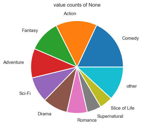
genre_val = pd.Series(genres_overall_df_1.values.flatten()).dropna()
plot_pie_value_counts(genre_val, 9)

# function to convert dataframe to long form for easier manipulation 

def convert_to_long(overall_df_1):
    
    public_score_series = top_anime_all_table[['id', 'public_score']].set_index('id')
    public_score_series

    df_stacked = overall_df_1.stack().to_frame()

    a = pd.DataFrame(df_stacked[0].values.tolist(), index = df_stacked.index)
    stacked_df = a.reset_index().drop(columns = ['level_1']).rename(columns={"level_0": "id", 0: "category"})
    b = stacked_df.set_index('id').join(public_score_series)

    return b

# function to plot category

def plot_category(b):
    
    sns.set(rc={'figure.figsize':(16,10)})
    sns.set_theme(style="whitegrid", palette="Set2")
    plt.xticks(rotation = 90)
    
    # Find the order
    my_order = b.groupby(by=["category"])["public_score"].mean().sort_values(ascending = False).index

    # plot boxplot
    sns.boxplot(data=b, x="category", y="public_score", order=my_order)

    plt.show()

genres_overall_long = convert_to_long(genres_overall_df_1)
demographics_overall_long = convert_to_long(demographics_overall_df_1)
themes_overall_long = convert_to_long(themes_overall_df_1)

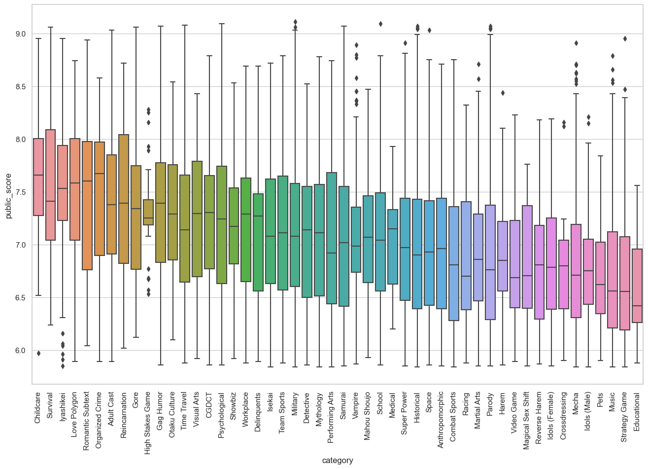
plot_category(themes_overall_long)

plot_category(genres_overall_long)

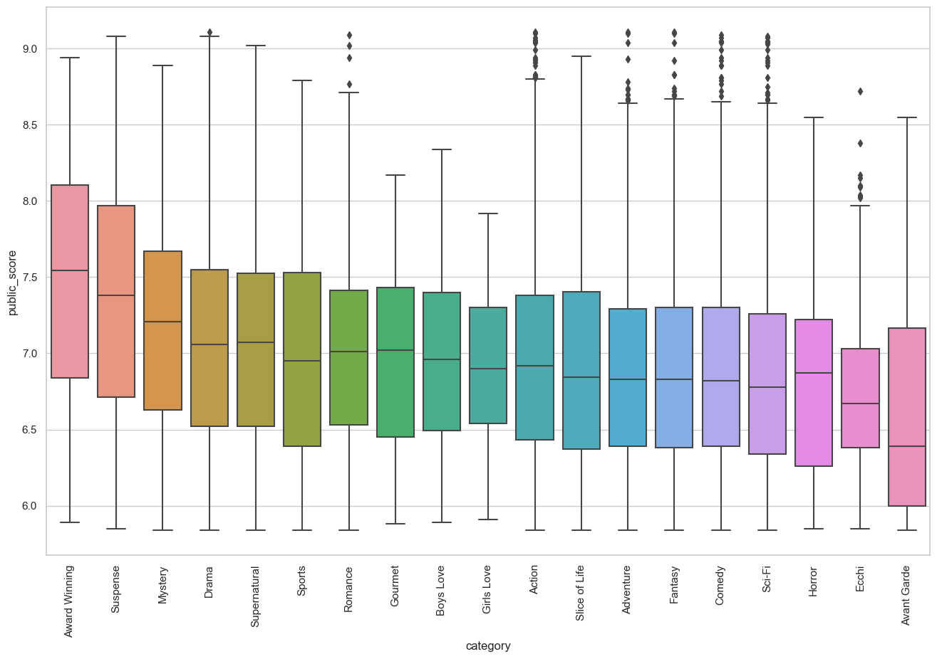
The above is a boxplot showing the average score of a show separated by genre. As expected, there seems to be minor differences in the average rating of the shows in relation to the genre. For instance, shows that have the “Award winning” genre score significantly better than those with “Avant Garde” genre. However, with the shows in the middle, it’s hard to tell a significant difference between the averages of the scores. For examples, genres such as mystery accounts for a small percentage of shows while shows with comedy as its genre can have an extremely wide range of ratings since people have different senses of humor. Due to the variance between the samples and the broad range that can be labeled with a genre, it is hard to attribute genre as a determining factor for the score of the anime.

Production Studio vs Score

# get list of studio by score. 

studios_s_1 = anime_info_frame_cleaned['studios'].dropna()
studios_df_1 = pd.DataFrame(item for item in studios_s_1).set_index(studios_s_1.index)
studios_overall_long = convert_to_long(studios_df_1)
studios_overall_long =studios_overall_long.rename(columns={"category": "studio"})

studio_mean_scores = studios_overall_long.groupby('studio').mean().sort_values(by = 'public_score', ascending = False)
studio_prod_counts = studios_overall_long['studio'].value_counts().rename('counts')#.head(50)

studio_avg_score_rank = studio_mean_scores.join(studio_prod_counts).reset_index()

print('------ Studios with highest average ranking anime ------\n  ')
display(studio_avg_score_rank.head(10))
print('------ Studios with highest average anime score with more than 20 animes produced ------\n  ')
studio_avg_score_rank[studio_avg_score_rank['counts'] > 20].head(20)

------ Studios with highest average ranking anime ------

	studio	public_score	counts
0	K-Factory	8.403333	3
1	Studio Bind	8.350000	3
2	Egg Firm	8.292500	4
3	Nippon Ramayana Film Co.	8.250000	1
4	Studio Signpost	8.060000	3
5	AHA Entertainment	7.920000	1
6	Studio Chizu	7.917500	4
7	Samsara Animation Studio	7.870000	1
8	Frontier One	7.850000	1
9	Studio Massket	7.800000	1

------ Studios with highest average anime score with more than 20 animes produced ------

	studio	public_score	counts
29	Kyoto Animation	7.433103	116
30	Wit Studio	7.425902	61
35	CloverWorks	7.383488	43
42	Bones	7.337361	144
43	White Fox	7.329070	43
45	David Production	7.322500	44
46	MAPPA	7.321475	61
55	ufotable	7.288906	64
57	Bandai Namco Pictures	7.287727	44
59	Lerche	7.265091	55
69	Shaft	7.235645	124
70	Studio Ghibli	7.234390	41
78	Trigger	7.203200	25
81	A-1 Pictures	7.199378	209
86	GoHands	7.186400	25
88	Seven Arcs	7.182857	28
92	Production I.G	7.177816	293
95	Manglobe	7.171935	31
98	P.A. Works	7.148367	49
100	8bit	7.135472	53

An initial assumption was made stating that certain studios can influence the rating of the show, hence, an investigation was done to see if the production studio can predict the quality of work. At first, it can be seen certain studios do have a much higher rating, however, this is because the studios have worked on a fewer anime which have scored high. Since there are many factors that go into the enjoyment of the show such as plot, voice acting etc., it is hard to pinpoint the studio is the main factor for the anime’s success. Thus, with a small sample size of shows produced, it is hard to say that these studios have a impact on the score. The above tables show a list of 20 studios which have produced over 25 anime along with their overall rank and average score of all the anime they produced. This table shows that if the studios that have produced less than 20 anime are removed, there is no major difference in the scores, with the first of which being “Kyoto Animations” which is already ranked 29th.

Designing the content recommendation system.

After the data has been cleaned and processed, the data can be used in a content recommendation system.

As mentioned previously, the concept of a content-filtering recommendation method is to find similar shows similar to the current one that a user is interested in. The general methodology is to convert the text to vector format and then use cosine similarity to generate similarity matrix. This matrix would simple be ranked and then read to extract the top recommended shows.

Again, the most relevant features need to be extracted. As explored in the previous sections, the most relevant information will be the following features of a given anime. The chosen features will include description, genres, studios, voice actors, staff, and characters as they are expected to have the highest impact when finding similar anime.

The following procedure is to eliminate the null values. Any record with a null value from any category will be removed. This reduced the sample size by 30%, from the initial 10,000 anime records to a total of 6,975 records. The reduction effect was mitigated as features with many missing values such as “themes” or “demographic” were removed. The remaining sample size is reasonable considering that all the values for every feature was retained. A sample of this table is shown.

anime_info_frame_cleaned
anime_info_frame_cleaned.isna().sum()
anime_info_f_master_fil = anime_info_frame_cleaned[['Type', 'Episodes', 'Status',
                                                    'aired_start', 'studios', 'source',
                                                    'genres_overall', 'duration_in_min', 
                                                    'public_score_rating','popularity']]

print('\n**** Filtered Frame NA counts ****\n')
print(anime_info_f_master_fil.isna().sum())
# dorp na values 
anime_info_f_master_fil_nona = anime_info_f_master_fil.dropna()

**** Filtered Frame NA counts ****

Type                      0
Episodes                  0
Status                    0
aired_start             199
studios                1227
source                    0
genres_overall          768
duration_in_min           8
public_score_rating       0
popularity                0
dtype: int64

### make dataframe columns with list to text and format for machine learning 

# display(all_anime_details_frame_no_nan_cvas)

### join characters, staff and VA to info dataframe 
anime_info_dataset_master1 = anime_info_f_master_fil_nona.join(all_anime_details_frame_no_nan_cvas , how = 'inner')
anime_info_dataset_master_lists = anime_info_dataset_master1[['studios', 'genres_overall', 
                                                              'characters',  'voice_actors', 'staff']]

anime_info_dataset_master_lists2 = anime_info_dataset_master_lists.applymap(lambda xs: ', '.join(str(x) for x in xs))
anime_info_dataset_master1[['studios', 'genres_overall','characters',  'voice_actors', 'staff']] = anime_info_dataset_master_lists2[['studios', 'genres_overall', 'characters',  'voice_actors', 'staff']]
ds = anime_info_dataset_master1.reset_index()
ds

	index	Type	Episodes	Status	aired_start	studios	source	genres_overall	duration_in_min	public_score_rating	popularity	characters	voice_actors	staff	description
0	5114	TV	64	Finished Airing	2009-04-05	Bones	Manga	Action, Adventure, Drama, Fantasy	24.0	9.111	3	Edward_Elric, Alphonse_Elric, Roy_Mustang, Mae...	Romi_Park, Rie_Kugimiya, Shinichiro_Miki, Keij...	Justin_Cook, Noritomo_Yonai, Yasuhiro_Irie, Ma...	After a horrific alchemy experiment goes wrong...
1	41467	TV	13	Currently Airing	2022-10-11	Pierrot	Manga	Action, Adventure, Fantasy	24.0	9.101	677	Ichigo_Kurosaki, Rukia_Kuchiki, Renji_Abarai, ...	Masakazu_Morita, Fumiko_Orikasa, Kentarou_Itou...	Tomohisa_Taguchi, Yukio_Nagasaki, Hikaru_Murat...	Substitute Soul Reaper Ichigo Kurosaki spends ...
2	43608	TV	13	Finished Airing	2022-04-09	A-1 Pictures	Manga	Comedy, Romance	23.0	9.091	239	Kaguya_Shinomiya, Yuu_Ishigami, Chika_Fujiwara...	Aoi_Koga, Ryouta_Suzuki, Konomi_Kohara, Makoto...	Shinichi_Omata, Jin_Aketagawa, Masakazu_Obara,...	The elite members of Shuchiin Academy's studen...
3	9253	TV	24	Finished Airing	2011-04-06	White Fox	Visual novel	Drama, Sci-Fi, Suspense	24.0	9.081	13	Rintarou_Okabe, Kurisu_Makise, Mayuri_Shiina, ...	Mamoru_Miyano, Asami_Imai, Kana_Hanazawa, Tomo...	Justin_Cook, Gaku_Iwasa, Takeshi_Yasuda, Shins...	Eccentric scientist Rintarou Okabe has a never...
4	28977	TV	51	Finished Airing	2015-04-08	Bandai Namco Pictures	Manga	Action, Comedy, Sci-Fi	24.0	9.071	337	Gintoki_Sakata, Kagura, Shinpachi_Shimura, Kot...	Tomokazu_Sugita, Rie_Kugimiya, Daisuke_Sakaguc...	Youichi_Fujita, Chizuru_Miyawaki, Shinji_Takam...	Gintoki, Shinpachi, and Kagura return as the f...
...	...	...	...	...	...	...	...	...	...	...	...	...	...	...	...
6936	8132	Movie	1	Finished Airing	2010-02-27	Sunrise	Original	Action	13.0	5.841	9944	Chouhi_Gundam, Kan-u_Gundam, Ryuubi_Gundam	Masayuki_Katou, Hiroki_Yasumoto, Yuuki_Kaji	Hiroyuki_Satou, Kenichi_Suzuki, Kunihiro_Mori,...	A Romance of the Three Kingdoms retelling usin...
6937	2754	OVA	3	Finished Airing	1989-04-28	J.C.Staff	Manga	Action, Adventure, Sci-Fi	37.0	5.841	8980	Cleopatra_Corns, Suen, Marianne, Dr_Randol, Na...	Maria_Kawamura, Hiromi_Tsuru, Yoshino_Takamori...	Kazuo_Katou, Naoyuki_Yoshinaga, Sukehiro_Tomit...	The Cleopatra Corns Group, aka Cleopatra DC, i...
6938	31318	TV	12	Finished Airing	2015-10-04	8bit	Original	Action, Adventure, Fantasy	23.0	5.841	1792	Felia, Mo_Ritika_Tzetzes_Ura, Sougo_Amagi, Kao...	Ayaka_Ohashi, Inori_Minase, Yuusuke_Kobayashi,...	Youhei_Kisara, Yasuhito_Kikuchi, Atsushi_Nakay...	In the world of Gift, the bowels of the planet...
6939	9862	Movie	1	Finished Airing	1992-08-08	Production Reed, Asahi Production	Original	Adventure, Fantasy	43.0	5.841	13444	Mary_Bell, Yuuri	Chieko_Honda, Satomi_Koorogi	Shigeyuki_Yamamori	Mary Bell, Yuri, Ken, Ribbon, and Tambourine g...
6940	34332	TV	12	Finished Airing	2019-01-11	Fukushima Gaina	Original	Comedy, Slice of Life	5.0	5.841	8489	Miku, Nagisa, Mona, Moe, Shiina, Suzu, Fumi, M...	Miku_Itou, Sarah_Emi_Bridcutt, Suzuko_Mimori, ...	Yoshinori_Asao, Kisuke_Koizumi, AOP, Ryouzou_O...	The anime will center on a group of young girl...

6941 rows × 15 columns

Building The Algorithm

About Tf-idf Vectorization

The selected columns of text were then converted to a vector format. For this, TfidfVectorizer in the sci-kit learn package in python was used. TfidfVectorizer is a class in scikit-learn that can be used to convert a collection of raw documents into a matrix of Tf-idf features. Tf-idf stands for term frequency-inverse document frequency, and it is a measure of the importance of a word in a document relative to a collection of documents. The goal of using Tf-idf is to down-weight the importance of words that are common to many documents and up-weight the importance of words that are rare or specific to a particular document. The process of TfidfVectorizer is as follows:

1. It tokenizes the input documents, meaning it breaks each document down into a list of individual words (also called tokens).
2. It removes stop words, which are words that are common and do not convey much meaning (e.g., “the,” “a,” “an”).
3. It computes the term frequency (tf) for each token, which is the number of times the token appears in a document.
4. It computes the inverse document frequency (idf) for each token, which is a measure of how rare the token is across the entire collection of documents.
5. It computes the Tf-idf score for each token, which is the product of the tf and idf scores.
6. It returns a matrix where each row represents a document and each column represents a token, and the cell value is the Tf-idf score for that token in that document.

About Cosine Similaritiy

In practical terms, cosine similarity is a measure of similarity between two vectors based on the angle between them. If the vectors are pointing in the same direction, their cosine similarity will be 1. If they are pointing in opposite directions, their cosine similarity will be -1. If the vectors are orthogonal to each other, their cosine similarity will be 0.

# return item name based on id 
def item(id1):  
    
    # display(top_anime_all_table[top_anime_all_table['id'] == id1])
    item_dis = top_anime_all_table.loc[top_anime_all_table['id'] == id1 ]

    return item_dis.loc[:,'Title'].item()
     

Building the function

A function was built to iterate through each record of the anime information table and find the most similar items computed by the cosine similarity function. The top 100 similar items were extracted then sorted, excluding the first entry as it would be the anime itself. These values were then stored in a dictionary, then converted into a table. A sample of this table can be shown in Figure 15 below, where “watch_id” is the watched show, and the “id” is the recommendation id along with its cosine similarity listed.

# convert words in array to vector format

def find_similarity_cosine(ds, column = 'description'):
    
    tf = TfidfVectorizer(analyzer='word', ngram_range=(1, 3), min_df=0, stop_words='english')
    tfidf_matrix = tf.fit_transform(ds[column])

    # find cosine similarity 
    cosine_similarities = cosine_similarity(tfidf_matrix, tfidf_matrix)

    # itterate through results and find similar 

    results = {}

    for idx, row in ds.iterrows():

        # sort top 100 
        similar_indices = cosine_similarities[idx].argsort()[:-100:-1] 
        # get similaries 
        similar_items = [(cosine_similarities[idx][i], ds['index'][i]) for i in similar_indices] 
        results[row['index']] = similar_items[1:]
        
        
    # convert to dataframe
    content_rec_des = pd.DataFrame.from_dict(results, orient="index").stack().to_frame()
    content_rec_des = pd.DataFrame(content_rec_des[0].values.tolist(), index = content_rec_des.index)

    content_rec_des = content_rec_des.reset_index(level=[0,1])

    content_rec_des = content_rec_des.rename(columns = {'level_0': 'watch_id' ,
                                                        'level_1' :'rec_no',
                                                        0 : 'cos_sim',
                                                        1: 'id'})

    content_rec_des['unique_key'] = content_rec_des['watch_id'].astype(str) + content_rec_des['id'].astype(str)

    return content_rec_des

def reccomend_content(results_df, a_id, number_of_rec): 
    
    a_df = results_df[results_df['watch_id'] == a_id]
    a_df_sort = a_df.sort_values(by = ['cos_sim'], ascending = False)
    
    anime_ids_list = list(a_df_sort['id'][:number_of_rec])
    
    # print('reccomendations for ' + item(a_id) + 'id = ' + str(a_id))
    
    display(top_anime_all_table[top_anime_all_table['id'] == a_id])
    
    return top_anime_all_table[top_anime_all_table['id'].isin(anime_ids_list)]

# generate similar series based on these categories. 
# plot / description seems to work the best. 
results_des = find_similarity_cosine(ds,'description')
results_genres = find_similarity_cosine(ds,'genres_overall')
results_stu = find_similarity_cosine(ds,'studios')
results_va = find_similarity_cosine(ds,'voice_actors')
results_staff = find_similarity_cosine(ds,'staff')
results_char = find_similarity_cosine(ds,'characters')

results_des

	watch_id	rec_no	cos_sim	id	unique_key
0	5114	0	0.158597	121	5114121
1	5114	1	0.089567	9135	51149135
2	5114	2	0.077452	430	5114430
3	5114	3	0.040949	6421	51146421
4	5114	4	0.026087	1266	51141266
...	...	...	...	...	...
680213	34332	93	0.017632	30988	3433230988
680214	34332	94	0.017347	1175	343321175
680215	34332	95	0.017303	17409	3433217409
680216	34332	96	0.017286	1254	343321254
680217	34332	97	0.017284	32171	3433232171

680218 rows × 5 columns

### manual checking 
# full metal alchemist id = 5114, 
# code geass id = 1575
# gintama id = 9969
# kimi no na wa, move id = 32281

an_id = 32281
by_des = reccomend_content(results_char, an_id, 5)
by_des

	Rank	Title	link	id	public_score	prive_rating	watch_status
24	25	Kimi no Na wa.	https://myanimelist.net/anime/32281/Kimi_no_Na_wa	32281	8.85	10.0	Completed

	Rank	Title	link	id	public_score	prive_rating	watch_status
238	239	Tenki no Ko	https://myanimelist.net/anime/38826/Tenki_no_Ko	38826	8.30	7.0	Completed
699	700	Kotonoha no Niwa	https://myanimelist.net/anime/16782/Kotonoha_n...	16782	7.91	NaN	Add to list
2568	2569	Blend S	https://myanimelist.net/anime/34618/Blend_S	34618	7.29	7.0	Completed
2639	2640	Slayers: The Motion Picture	https://myanimelist.net/anime/536/Slayers__The...	536	7.28	NaN	Add to list
2648	2649	Watashi ni Tenshi ga Maiorita! Special	https://myanimelist.net/anime/38999/Watashi_ni...	38999	7.28	NaN	Add to list

Content Filtering Results Discussion

The recommendation was also computed but with characters, genres, studios, voice actors and staff . A breakdown is listed for each below.

• Description: Finding the cosine similarity for description seems to produce the best results. This is most likely because the description has the most words, hence the algorithm can find similar series better than the other features. However, as mentioned, as it simply finds the term frequency and may not recommend actually similar plotlines.
• Genres: Due to the limited words given, the algorithm will recommend the first series that has an exact match with the show’s current genre. Genres is generally not a good metric to use, however, it might be useful if the user shows interest in a certain genre. This can be combined with the public score to randomly recommend the top-rated one of the genre.
• Studio: This category interacts in the same as it does with Genre, where the algorithm finds the closest match, for example, “Code Geass” is produced by Sunrise studio, and the algorithm will find the first 5 series with the same studio. Although “Code Geass R2” is the direct sequel, it didn’t recommend it. As investigated previously, the studio does not correlate to any specific genre or the overall quality of the show and thus is not a good feature to find similarities between shows.
• Voice actors. Similar voice actors often voice characters in related series, and this is also the case with movies. Some voice actors carry over to similar roles across movies, which makes voice actors a decent choice to find similar anime.
• Staff: The same concept applies to staff As seen in the anime “Your Name” the top recommendations are “Tenki no ko” and “Suzume no Tojimari”, which are all highly rated anime movies produced by director “Makoto Shinkai”. The art style, music, and style are quite similar to one another, which can make staff a decent correlating factor when finding similar series.
• Characters: Using the characters in the show are perfect for finding a sequel, and in some cases, might even be more accurate than the description given its low word density. However, this feature may severely lack in terms when a standalone movie is introduced as there are no shared characters.

Although content-based recommendation systems will always recommend similar items, which the user would have a high chance to enjoy, the weakness is that this system leaves no room to discover new shows. For instance, most of the series that are recommended are sequels to the originals, however, it is not as good as recommending series that are outside this range. This would ultimately lead to a repetitive user experience, hence the need for collaborative filtering.

Collaborative filtering approach

Collaborative filtering is a method of recommending items to users based on the preferences of similar users. It works by identifying users who have similar preferences and uses those preferences to recommend items to the active user. There are two main types of collaborative filtering systems:

• Memory-based collaborative filtering: This method uses the entire user-item dataset to compute the similarity between users or items and make recommendations. The advantage of this approach is that it can make recommendations for any item, even those that are new or have no ratings yet. The disadvantage is that it may be computationally expensive and may not scale well with a very large dataset.
• Model-based collaborative filtering: This method uses machine learning techniques to learn the relationships between different users and items and make recommendations. The advantage of this approach is that it can scale better with a large dataset and may be able to provide more accurate recommendations. The disadvantage is that it may be more difficult to implement and may not be able to make recommendations for new or unrated items.

This notebook will investigate model-based collaborative filtering. One of the advantages of a model-based collaborative filtering system is that it does not need to rely on understanding the item content. A major downside to this method is the cold start problem, where the system does not recommend new items well when there has been no user-item interaction with it. This implies that the sample size and database must be very robust in order to make an accurate prediction.

This notebook will also be using user data scraped from myanimelist, the code for which can be found under another notebook

import numpy as np
from bs4 import BeautifulSoup
import requests
import re
import requests
import lxml.html as lh
import pandas as pd
import pickle
import os 
import scipy.stats as stats
import seaborn as sns
import matplotlib.pyplot as plt

pd.options.mode.chained_assignment = None  # default='warn'

top_anime_all_table = pd.read_csv('/Users/rayenfeng/Documents/code/anime_rec_project/data_sources_pickle/all_anime_directory.csv')
top_anime_all_table.head()

	Rank	Title	link	id	public_score	prive_rating	watch_status
0	1	Fullmetal Alchemist: Brotherhood	https://myanimelist.net/anime/5114/Fullmetal_A...	5114	9.11	10.0	Completed
1	2	Bleach: Sennen Kessen-hen	https://myanimelist.net/anime/41467/Bleach__Se...	41467	9.10	NaN	Add to list
2	3	Kaguya-sama wa Kokurasetai: Ultra Romantic	https://myanimelist.net/anime/43608/Kaguya-sam...	43608	9.09	10.0	Completed
3	4	Steins;Gate	https://myanimelist.net/anime/9253/Steins_Gate	9253	9.08	10.0	Completed
4	5	Gintama°	https://myanimelist.net/anime/28977/Gintama°	28977	9.07	NaN	Completed

# import scraped user information. 

all_user_rating_df1 = pd.read_csv('/Users/rayenfeng/Documents/code/anime_rec_project/data_sources_pickle/all_user_anime_ratings.csv')
all_user_rating_df1 = all_user_rating_df1.rename(columns = {'level_0' : 'username', 'level_1': 'sub_link', '0': 'user_rating'})

# import data scrape from the second file 

all_user_rating_df2 = pd.read_csv('/Users/rayenfeng/Documents/code/anime_rec_project/data_sources_pickle/all_user_anime_ratings2.csv')
all_user_rating_df2 = all_user_rating_df2.rename(columns = {'level_0' : 'username', 'level_1': 'sub_link', '0': 'user_rating'})

# combine both dataframes. 

all_user_rating_df = pd.concat([all_user_rating_df1, all_user_rating_df2], axis=0)
all_user_rating_df

	username	sub_link	user_rating
0	tazillo	/anime/47/Akira	5
1	tazillo	/anime/6547/Angel_Beats	3
2	tazillo	/anime/9989/Ano_Hi_Mita_Hana_no_Namae_wo_Bokut...	-
3	tazillo	/anime/11111/Another	2
4	tazillo	/anime/477/Aria_the_Animation	-
...	...	...	...
678738	neongenesis92i	/anime/1251/Fushigi_no_Umi_no_Nadia	9
678739	sarah501689	/anime/40421/Given_Movie	10
678740	aReallyBigFan	/anime/38088/Digimon_Adventure__Last_Evolution...	10
678741	MauvaiseHerbe	/anime/40911/Yuukoku_no_Moriarty	3
678742	Storm9265	/anime/32005/Detective_Conan_Movie_20__The_Dar...	1

1596003 rows × 3 columns

Dataset Cleaning

# extract user ids into seperate column 

all_user_rating_df['id'] =  all_user_rating_df['sub_link'].apply(lambda x: int(x.split('/')[2]))

#print number of unique ids and animes
print('******* the number of unique users: ' + str(len(all_user_rating_df['username'].unique())) + ' *******\n')
print('******* the number of unique animes: ' + str(len(all_user_rating_df['id'].unique())) + ' *******\n')

### '-' means that user has not finished watching the show, can replace with nan. 
all_user_rating_df['user_rating'] = all_user_rating_df['user_rating'].replace('-', np.nan)

all_user_rating_df_no_null = all_user_rating_df.dropna()

print('******* null values: *******\n') 
print(all_user_rating_df_no_null.isna().sum())

all_user_rating_df_no_null_test = all_user_rating_df_no_null.copy()
all_user_rating_df_no_null_test.head()

******* the number of unique users: 4521 *******

******* the number of unique animes: 19056 *******

******* null values: *******

username       0
sub_link       0
user_rating    0
id             0
dtype: int64

	username	sub_link	user_rating	id
0	tazillo	/anime/47/Akira	5	47
1	tazillo	/anime/6547/Angel_Beats	3	6547
3	tazillo	/anime/11111/Another	2	11111
5	tazillo	/anime/7817/B-gata_H-kei	5	7817
6	tazillo	/anime/5081/Bakemonogatari	7	5081

# import my ratings.  

my_ratings1 = top_anime_all_table.dropna(subset = ['prive_rating'])
my_ratings2 = my_ratings1[['link', 'id', 'prive_rating']]
my_ratings2['username'] = 'Destinyflame'
my_ratings2['sub_link'] = my_ratings2['link'].apply(lambda x: x.replace('https://myanimelist.net', ''))
my_ratings3 = my_ratings2.drop(columns=['link'])
my_ratings3 = my_ratings3[['username', 'sub_link', 'prive_rating', 'id']].rename(columns = {'prive_rating': 'user_rating'})


display(my_ratings3)

print('\n ******* null values: *******\n') 
print(all_user_rating_df_no_null.isna().sum())

	username	sub_link	user_rating	id
0	Destinyflame	/anime/5114/Fullmetal_Alchemist__Brotherhood	10.0	5114
2	Destinyflame	/anime/43608/Kaguya-sama_wa_Kokurasetai__Ultra...	10.0	43608
3	Destinyflame	/anime/9253/Steins_Gate	10.0	9253
5	Destinyflame	/anime/38524/Shingeki_no_Kyojin_Season_3_Part_2	10.0	38524
8	Destinyflame	/anime/15417/Gintama__Enchousen	10.0	15417
...	...	...	...	...
5904	Destinyflame	/anime/36407/Kenja_no_Mago	6.0	36407
6529	Destinyflame	/anime/34934/Koi_to_Uso	6.0	34934
7001	Destinyflame	/anime/38610/Tejina-senpai	5.0	38610
7282	Destinyflame	/anime/36511/Tokyo_Ghoul_re	7.0	36511
7307	Destinyflame	/anime/32901/Eromanga-sensei	7.0	32901

298 rows × 4 columns

 ******* null values: *******

username       0
sub_link       0
user_rating    0
id             0
dtype: int64

# combined my ratings with all user ratings
combined_anime_data = pd.concat([all_user_rating_df_no_null_test, my_ratings3], axis=0)

# keep anime with more than 25 review
combined_anime_data['reviews'] = combined_anime_data.groupby(['id'])['user_rating'].transform('count')

# diplay(combined_anime_data)

combined_anime_data1 = combined_anime_data[combined_anime_data['reviews'] > 25]

combined_anime_data2 = combined_anime_data1[['username', 'id', 'user_rating']].astype({'user_rating': 'int64'})
combined_anime_data2

	username	id	user_rating
0	tazillo	47	5
1	tazillo	6547	3
3	tazillo	11111	2
5	tazillo	7817	5
6	tazillo	5081	7
...	...	...	...
5904	Destinyflame	36407	6
6529	Destinyflame	34934	6
7001	Destinyflame	38610	5
7282	Destinyflame	36511	7
7307	Destinyflame	32901	7

1262257 rows × 3 columns

Training the first reccomendation model

from surprise import NMF, SVD, SVDpp, KNNBasic, KNNWithMeans, KNNWithZScore, CoClustering, NormalPredictor
from surprise.model_selection import cross_validate
from surprise import Reader, Dataset

reader = Reader(rating_scale=(1, 10))
data = Dataset.load_from_df(combined_anime_data2, reader)

# get the list of the anime ids
unique_ids = combined_anime_data2['id'].unique()
# get the list of the ids that the username destinyflame has rated
ids_user_destinyflame = combined_anime_data2.loc[combined_anime_data2['username'] == 'Destinyflame', 'id']

# remove the rated movies for the recommendations
animes_to_predict = np.setdiff1d(unique_ids , ids_user_destinyflame)

# define funciton that predicts how the user would score anime 
# inputs are username as string and algorithm as suprise algo, default is set to NMF. 

def find_user_reccomednations(user_name, algorithm = NMF()): 
    
    algo = algorithm
    algo.fit(data.build_full_trainset())
    my_recs = []

    for i_id in animes_to_predict:
        
        my_recs.append((i_id, algo.predict(uid = user_name ,iid = i_id).est))

    my_recs_df = pd.DataFrame(my_recs, columns = ['anime_ids', 'predictions']).sort_values('predictions', ascending=False)
    
    return my_recs_df

# NMF, SVD, SVDpp, KNNBasic, KNNWithMeans, KNNWithZScore, CoClustering, NormalPredictor

display(find_user_reccomednations('Destinyflame', SVD()))

	anime_ids	predictions
3590	28977	9.787165
2397	9969	9.555680
5168	42938	9.422987
4821	39486	9.370195
4289	35247	9.368408
...	...	...
2769	13405	3.064923
325	413	2.769959
4758	38853	2.754034
4048	33394	2.599562
1596	3287	2.403478

5476 rows × 2 columns

# Previewing results
top_anime_all_table[top_anime_all_table['id'].isin([50160, 28977])]

	Rank	Title	link	id	public_score	prive_rating	watch_status
4	5	Gintama°	https://myanimelist.net/anime/28977/Gintama°	28977	9.07	NaN	Completed
38	39	Kingdom 4th Season	https://myanimelist.net/anime/50160/Kingdom_4t...	50160	8.77	NaN	Add to list

Thoughts on previewed results:

it’s a good thing that it thinks i’ll like gintama, I probably watched this series and didn’t update the score. As seen in this image, the status is completed, but I forgot to score it, if I did, it would be a 9 or 10 because Gintama is one of my favourite shows

Comparing algorithms for collaborative filtering (improving results)

With each dataframe method, there is bound to be some sort of error within the predicted value and the actual value. For this, each reccomendation algorythm can be evaluated by first splitting the data into two subsets; the test and train dataframe. The training dataset will be used to train the algoythm. Then this algorythm will be applyed to the test dataset and will predict a rating. The accuracy with the actual score in the test datset will be computed.

Python Surprise package default cross-validation system splits the data using and runs a cross validation x times. Then gets the RSME, which is the root squared mean error. The second measure is MAE, which is the Mean of Absolute value of Errors. The lower the number the better.

For this segment, a recommendation system will be built with the surprise package in Python which is a package for building and analyzing recommender systems that deal with explicit rating data. After importing the packages, a simple function was built that predicts the score, given a username and a certain algorithm. The recommendation system will then be tested using 5 different recommendation algorithms, and these algorithms will be evaluated based on their prediction accuracy. The implementation of these algorithms will be focused on, as the mathematics behind them are complex in nature and a deep dive into them is beyond the score of this project, hence a brief description will be given below of each algorithm used.

• SVD: Singular Value Decomposition is an algorithm that takes a matrix and decomposes it into three smaller matrices that represent the underlying structure of the original matrix. These three matrices can be used to reconstruct the original matrix, and they provide a way to understand the relationships between the rows and columns of the original matrix.
• NMF: Non-Negative Matrix Factorization is similar to other matrix factorization techniques, such as Singular Value Decomposition (SVD), but it has the additional constraint that the matrices it decomposes must be non-negative.
• SVDpp: Singular Value Decomposition ++ is an algorithm identical to SVD however it takes into account implicit ratings.
• KNNWithZScore: K-Nearest Neighbors with Z-score normalization is a machine learning approach that involves applying KNN to a dataset where the features have been standardized using the Z-score method. It is often used to improve the performance of the KNN algorithm by ensuring that the features are on the same scale and have similar statistical properties.
• CoClustering: Co-clustering is a machine learning technique that involves simultaneously clustering the rows and columns of a matrix. It is a form of clustering that can be used to find patterns and structures in data that is arranged in a matrix format.

More on cross validation, MAE and RMSE.

Cross-validation is a resampling procedure used to evaluate a machine learning model on a limited data sample. The goal of cross-validation is to tune the parameters (i.e., the hyperparameters) of a model in a way that maximizes the model’s ability to predict the target variable. The algorithms will be validated with the k-fold cross validation technique.

In k-fold cross-validation, the data sample is randomly partitioned into k smaller sets, or folds. The model is trained on k-1 folds and tested on the remaining fold. This process is repeated k times, with a different fold being used as the test set each time. The performance measure is then averaged across all k iterations.

The average performance of the algorithms will be measured using MAE and RMSE. The computation time will also be considered during the evaluation but is not the main focus. MAE and RMSE are two different metrics that can be used to evaluate the performance of a machine-learning model during cross-validation.

MAE stands for mean absolute error. It is a measure of the average absolute difference between the predicted values and the true values. It is calculated as the sum of the absolute differences between the predicted and true values, divided by the total number of predictions. MAE is a simple and easy-to-understand metric, but it is sensitive to outliers because it does not square the differences before taking the mean. Equation (3 is the mathematical formula for MAE.

RMSE stands for root mean squared error. It is a measure of the average squared difference between the predicted values and the true values. It is calculated as the square root of the mean squared error (MSE), which is the average of the squared differences between the predicted and true values. RMSE is more sensitive to outliers than MAE because it squares the differences before taking the mean. Equation (4 is the mathematical formula for RMSE.

In general, a model with a lower MAE or RMSE is considered to be a better model because it is making predictions that are closer to the true values.

cross_validation_score = {}
# Iterate over all recommender system algorithms

for rec_system in [NMF(), SVD() , SVDpp(), KNNWithZScore(), CoClustering()]:
    
    # Perform cross validation
    
    cross_val_df = cross_validate(rec_system, data, cv = 3)
    method_name = str(rec_system).split(' ')[0].split('.')[-1]
    cross_validation_score[method_name] = cross_val_df
    
    

Computing the msd similarity matrix...
Done computing similarity matrix.
Computing the msd similarity matrix...
Done computing similarity matrix.
Computing the msd similarity matrix...
Done computing similarity matrix.

cross_val_df_all_method = pd.DataFrame.from_dict(cross_validation_score, orient='index')
cross_val_df_all_method_means = cross_val_df_all_method.applymap(lambda x: np.array(x).mean())

cross_val_df_all_method_means.sort_values(by=['test_rmse'])

	test_rmse	test_mae	fit_time	test_time
SVD	1.285141	0.955953	9.375140	3.445283
SVDpp	1.328549	0.989146	422.367654	185.372463
KNNWithZScore	1.367502	1.026495	25.286533	170.895483
CoClustering	1.424752	1.070978	19.545526	3.579695
NMF	1.913623	1.613487	16.732938	3.112131

The best performing algorithm is SVD and it also has the lowest fit time. Therfore, the SVD algorithm will be run.

ranked_user_reccomendations_df = find_user_reccomednations('Destinyflame', SVD())
# display(ranked_user_reccomendations_df)
top_anime_all_table[top_anime_all_table['id'].isin(ranked_user_reccomendations_df['anime_ids'][:50])]

	Rank	Title	link	id	public_score	prive_rating	watch_status
4	5	Gintama°	https://myanimelist.net/anime/28977/Gintama°	28977	9.07	NaN	Completed
6	7	Gintama'	https://myanimelist.net/anime/9969/Gintama	9969	9.05	NaN	Completed
7	8	Gintama: The Final	https://myanimelist.net/anime/39486/Gintama__T...	39486	9.05	NaN	Add to list
11	12	Fruits Basket: The Final	https://myanimelist.net/anime/42938/Fruits_Bas...	42938	9.02	NaN	Add to list
13	14	3-gatsu no Lion 2nd Season	https://myanimelist.net/anime/35180/3-gatsu_no...	35180	8.95	NaN	Add to list
22	23	Owarimonogatari 2nd Season	https://myanimelist.net/anime/35247/Owarimonog...	35247	8.89	NaN	Add to list
31	32	Kizumonogatari III: Reiketsu-hen	https://myanimelist.net/anime/31758/Kizumonoga...	31758	8.80	NaN	Add to list
32	33	Bocchi the Rock!	https://myanimelist.net/anime/47917/Bocchi_the...	47917	8.79	NaN	Add to list
40	41	Hajime no Ippo	https://myanimelist.net/anime/263/Hajime_no_Ippo	263	8.75	NaN	Add to list
41	42	Mushishi Zoku Shou 2nd Season	https://myanimelist.net/anime/24701/Mushishi_Z...	24701	8.74	NaN	Add to list
47	48	Rurouni Kenshin: Meiji Kenkaku Romantan - Tsui...	https://myanimelist.net/anime/44/Rurouni_Kensh...	44	8.71	NaN	Add to list
53	54	Fate/stay night Movie: Heaven's Feel - III. Sp...	https://myanimelist.net/anime/33050/Fate_stay_...	33050	8.69	NaN	Add to list
55	56	One Piece	https://myanimelist.net/anime/21/One_Piece	21	8.68	NaN	Dropped
61	62	Hajime no Ippo: New Challenger	https://myanimelist.net/anime/5258/Hajime_no_I...	5258	8.66	NaN	Add to list
66	67	Mob Psycho 100 III	https://myanimelist.net/anime/50172/Mob_Psycho...	50172	8.65	NaN	Add to list
72	73	Tengen Toppa Gurren Lagann	https://myanimelist.net/anime/2001/Tengen_Topp...	2001	8.63	NaN	Add to list
78	79	Seishun Buta Yarou wa Yumemiru Shoujo no Yume ...	https://myanimelist.net/anime/38329/Seishun_Bu...	38329	8.61	NaN	Add to list
81	82	Hajime no Ippo: Rising	https://myanimelist.net/anime/19647/Hajime_no_...	19647	8.59	NaN	Add to list
82	83	JoJo no Kimyou na Bouken Part 5: Ougon no Kaze	https://myanimelist.net/anime/37991/JoJo_no_Ki...	37991	8.58	NaN	Add to list
83	84	Kizumonogatari II: Nekketsu-hen	https://myanimelist.net/anime/31757/Kizumonoga...	31757	8.58	NaN	Add to list
90	91	Spy x Family Part 2	https://myanimelist.net/anime/50602/Spy_x_Fami...	50602	8.57	NaN	Add to list
104	105	Bakuman. 3rd Season	https://myanimelist.net/anime/12365/Bakuman_3r...	12365	8.54	NaN	Add to list
119	120	Fate/stay night Movie: Heaven's Feel - II. Los...	https://myanimelist.net/anime/33049/Fate_stay_...	33049	8.51	NaN	Add to list
135	136	Mahou Shoujo Madoka★Magica Movie 3: Hangyaku n...	https://myanimelist.net/anime/11981/Mahou_Shou...	11981	8.47	NaN	Add to list
143	144	Steins;Gate Movie: Fuka Ryouiki no Déjà vu	https://myanimelist.net/anime/11577/Steins_Gat...	11577	8.46	NaN	Add to list
148	149	Zoku Owarimonogatari	https://myanimelist.net/anime/36999/Zoku_Owari...	36999	8.45	NaN	Add to list
153	154	JoJo no Kimyou na Bouken Part 3: Stardust Crus...	https://myanimelist.net/anime/26055/JoJo_no_Ki...	26055	8.44	NaN	Add to list
162	163	Major S5	https://myanimelist.net/anime/5028/Major_S5	5028	8.41	NaN	Add to list
172	173	Kara no Kyoukai Movie 7: Satsujin Kousatsu (Go)	https://myanimelist.net/anime/5205/Kara_no_Kyo...	5205	8.40	NaN	Add to list
188	189	Kizumonogatari I: Tekketsu-hen	https://myanimelist.net/anime/9260/Kizumonogat...	9260	8.37	NaN	Add to list
198	199	Re:Zero kara Hajimeru Isekai Seikatsu 2nd Season	https://myanimelist.net/anime/39587/Re_Zero_ka...	39587	8.35	NaN	Add to list
199	200	Bakuman. 2nd Season	https://myanimelist.net/anime/10030/Bakuman_2n...	10030	8.35	NaN	Add to list
203	204	Gotcha!	https://myanimelist.net/anime/42984/Gotcha	42984	8.34	NaN	Add to list
220	221	Katanagatari	https://myanimelist.net/anime/6594/Katanagatari	6594	8.32	NaN	Add to list
222	223	Kemono no Souja Erin	https://myanimelist.net/anime/5420/Kemono_no_S...	5420	8.32	NaN	Add to list
239	240	World Trigger 3rd Season	https://myanimelist.net/anime/44940/World_Trig...	44940	8.30	NaN	Add to list
271	272	Stranger: Mukou Hadan	https://myanimelist.net/anime/2418/Stranger__M...	2418	8.27	NaN	Add to list
279	280	JoJo no Kimyou na Bouken Part 6: Stone Ocean	https://myanimelist.net/anime/48661/JoJo_no_Ki...	48661	8.26	NaN	Add to list
292	293	Gyakkyou Burai Kaiji: Hakairoku-hen	https://myanimelist.net/anime/10271/Gyakkyou_B...	10271	8.25	NaN	Add to list
295	296	Detective Conan: Episode One - The Great Detec...	https://myanimelist.net/anime/34036/Detective_...	34036	8.24	NaN	Add to list
417	418	Boku no Hero Academia 2nd Season	https://myanimelist.net/anime/33486/Boku_no_He...	33486	8.13	NaN	Watching
420	421	Mahou Shoujo Lyrical Nanoha: The Movie 2nd A's	https://myanimelist.net/anime/10153/Mahou_Shou...	10153	8.13	NaN	Add to list
428	429	Chuunibyou demo Koi ga Shitai! Movie: Take On Me	https://myanimelist.net/anime/35608/Chuunibyou...	35608	8.12	NaN	Add to list
450	451	One Piece Film: Strong World	https://myanimelist.net/anime/4155/One_Piece_F...	4155	8.10	NaN	Add to list
454	455	Tsukimonogatari	https://myanimelist.net/anime/28025/Tsukimonog...	28025	8.10	NaN	Add to list
541	542	Kara no Kyoukai Movie 3: Tsuukaku Zanryuu	https://myanimelist.net/anime/3783/Kara_no_Kyo...	3783	8.03	NaN	Add to list
625	626	One Piece Film: Red	https://myanimelist.net/anime/50410/One_Piece_...	50410	7.96	NaN	Add to list
658	659	Clannad: Mou Hitotsu no Sekai, Tomoyo-hen	https://myanimelist.net/anime/4059/Clannad__Mo...	4059	7.94	NaN	Add to list
686	687	Code Geass: Fukkatsu no Lelouch	https://myanimelist.net/anime/34437/Code_Geass...	34437	7.92	NaN	Add to list
2906	2907	Darling in the FranXX	https://myanimelist.net/anime/35849/Darling_in...	35849	7.22	NaN	Add to list

Yay, I got more shows to watch.

Well, I hope all this work was worth it, just to find some anime to watch. It’ll be annoying to update this dataset each time, so I hope I can find a way to integrate this with something else.

Final Approach Discussion

As explored, collaborative filtering and content-based filtering are two different techniques used to make recommendations in a recommendation system.

Content-based filtering is a method of making recommendations based on the characteristics of the items being recommended. In order for it to do so, content-based filtering algorithms require information about the items being recommended, such as their features, descriptions, or genres.

Collaborative filtering is a method of making recommendations based on the preferences of similar users by identifying users who have similar tastes and preferences and using those preferences to make recommendations to the current user. A strength of collaborative filtering algorithms is that it does not require any information about the items being recommended. In this case, only the user, anime id, and score were given to produce accurate recommendations.
Both collaborative filtering and content-based filtering have their own strengths and weaknesses. Collaborative filtering can make personalized recommendations based on the preferences of similar users, but it may struggle to make recommendations for users who are new to the system or who have few ratings. Content-based filtering can make recommendations based on the characteristics of the items, but it may struggle to capture complex relationships between items or to make recommendations that are outside the user’s usual interests.

In this case, given the already robust database that myanimelist.net has, both approaches would have no restrictions if they were implemented, although a collaborative filtering approach seems to be produce more accurate results and is the favoured approach to use. However, based on the results of this study, a hybrid approach may need to be used to take the strengths of each method.

Conclusion

This report compared content based and collaborative recommendation systems. For content-based systems, a model-based system was used. The database contained 10,000 anime and their data such as genres, characters, and descriptions. During the data exploration, outliers were found and it could be seen that no feature is a definite predictor of score. This process also identified five key features; description, genres, characters, staff, and voice actors which are expected to relate similar items. The cosine similarity between animes was found for each of the features and similar items were computed for each feature. It was found that content-based recommendation method was very proficient at find sequels of shows, however, as it searches by keywords and term frequency, it may ultimately lead to a repetitive user experience

For a collaborative filtering method, information from over 4000 unique users containing 1.5 million anime ratings were gathered. Five different algorithms were cross validated and the SVD algorithm performed the best and was implemented into the system. The results were investigated using a sample user, and the results from this method were accurate in their predictions.

Reccomendations (haha get it?) on further work

The following section is outlined for the further development of the anime recommendation system. In this study, a user-user based method was used for collaborative filtering and a model-based method was used for content filtering. For the future, it can be good to strengthen the system by exploring an item-item based collaborative approach and a memory-based approach to content approach. Additionally, packages such as scikit learn and surprise were used, but a different approach such as using deep learning algorithms in the TensorFlow package might also provide good insight. Although it was outside the score of the project, a good addition may be to make the system interactive, and web based. By making this web-based, it can synchronize with the database which would increase user and item information. This increase in information can be ultimately used to make better recommendations using a hybrid method which combines the two systems and their strengths.

References:

https://heartbeat.comet.ml/recommender-systems-with-python-part-i-content-based-filtering-5df4940bd831 https://towardsdatascience.com/hands-on-content-based-recommender-system-using-python-1d643bf314e4 https://heartbeat.comet.ml/recommender-systems-with-python-part-i-content-based-filtering-5df4940bd831 https://towardsdatascience.com/hands-on-content-based-recommender-system-using-python-1d643bf314e4
https://predictivehacks.com/how-to-run-recommender-systems-in-python/

Suprise Python Documentaion:
https://surprise.readthedocs.io/en/stable/index.html

For information on prediction algorithms package:
https://surprise.readthedocs.io/en/stable/prediction_algorithms_package.html

MAE and RMSE documentation https://towardsdatascience.com/what-are-rmse-and-mae-e405ce230383#:~:text=Technically%2C%20RMSE%20is%20the%20Root,actual%20values%20of%20a%20variable.